5. User-Defined Functions#

5.1. Landmarks#

5.1.1. Some Definitions#

In previous chapters we made a distinction between the functions and operators which are part of APL, like +, ×, ⌈ and / (we refer to them as primitives), and those functions and operators that are created by the user which are represented, not by a symbol, but by a name like Average (we say they are user-defined).

We also made an important distinction between functions, which apply to data and which return data, and operators, which apply to functions or data and produce derived functions (see Section 4.8.2).

This means that we can distinguish between 4 major categories of processing tools:

Category	Name	Examples	Refer to
Built-in tools	Primitive functions	`+` `×` `⌈` `⍴`	Previous chapters
	Primitive operators	`/`	Chapter on operators
User-defined tools	User-defined functions	`Average`	This chapter
	User-defined operators		Section 11.13

This chapter is devoted to user-defined functions. The subject of user-defined operators will be covered later.

We can further categorise user-defined functions according to the way they process data. Firstly we can distinguish between direct and procedural functions:

direct functions (commonly referred to as dfns) are defined in a very formal manner; they are usually designed for pure calculation, without any external or user interfaces. Dfns do not allow loops except by recursion and have limited options for conditional programming; and
procedural functions (commonly referred to as tradfns, short for traditional functions) are less formal and look much more like programs written in other languages; they provide greater flexibility for building major applications which involve user interfaces, access to files or databases and other external interfaces. Tradfns may take no arguments and behave like scripts.

Even though you may write entire systems with dfns, you might prefer to restrict their use to encapsulate statements that, together, perform some meaningful operation on the data given. We will start by covering the syntax and characteristics of dfns, then we will do the same for tradfns, and then Section 5.8 will compare the main characteristics of both of them, to help you understand when and why each should be used.

The second distinction we can make concerns the number of arguments a user-defined function can have.

dyadic functions take two arguments which are placed on either side of the function (X f Y);
monadic functions take a single argument which is placed to the right of the function (f Y);
niladic functions take no argument at all; and
ambivalent functions are dyadic functions whose left argument is optional.

5.1.2. Configure Your Environment#

Dyalog APL has a highly configurable development and debugging environment, designed to fit the requirements of very different kinds of programmers. This environment is controlled by configuration parameters; let us determine which context will suit you best.

5.1.2.1. What Do You Need?#

All you need (except for love) is:

a window in which to type expressions that you want to be executed (white Session window);
one or more windows in which to create/modify user-defined functions (grey Edit windows); and
one or more windows to debug execution errors (black Trace window).

The colours above refer to the positions of the windows in Fig. 5.1, Fig. 5.2, and Fig. 5.3.

The default configuration is consistent with other software development tools and in it is possible to divide the session window into three parts which can be resized, as shown in Fig. 5.1:

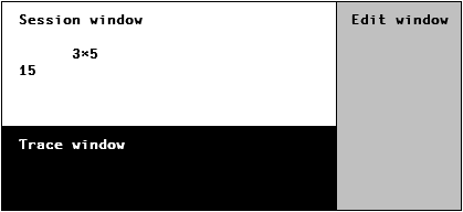
Fig. 5.1 The default window configuration.#

This configuration provides a single Edit window and a single Trace window, each of which is “docked” along one of the Session window borders. You can dock these windows along any of the Session window sides. For example, Fig. 5.2 shows a configuration with three horizontal panes, highly suitable for entering and editing very long statements.

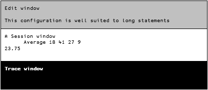
_images/IDE_Window_Horizontal_Layout.png

Fig. 5.2 The Edit and Trace windows in a horizontal layout.#

The Edit window supports the Multiple Document Interface (MDI). This means that you can work on more than one function at a time:

on the Windows interpreter you can use the “Window” menu to Tile and Cascade, or you can maximise any one of the functions to concentrate solely upon it; or
if you are using RIDE the default behaviour is to open a tab per item you are editing.

If you are working on a relatively small screen you may find that you prefer to work with “floating” windows in a layout similar to the one in Fig. 5.3:

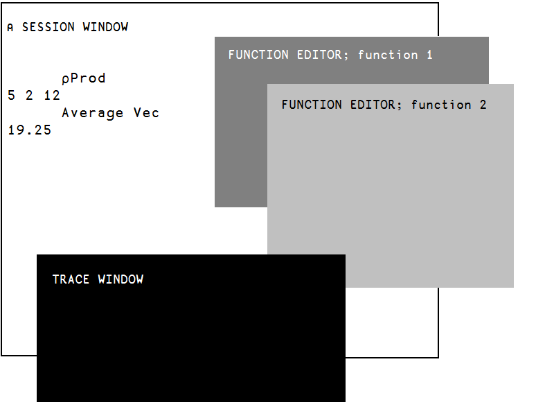
Fig. 5.3 “floating” windows layout.#

on the Windows interpreter, you can either:
- grab the border of a sub-window (Edit or Trace) and then drag and drop it in the middle of the session window, as an independent floating window; or
- enable the “Classic Dyalog mode”, which can be set under “Options” ⇨ “Configure…” ⇨ “Trace/Edit” as shown in Fig. 5.4.

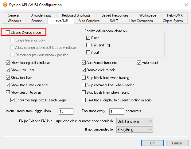
Fig. 5.4 Option to set “Classic Dyalog mode”.#

if you are using RIDE you can go to “Edit” ⇨ “Preferences” ⇨ “Windows” and enable “Floating windows” as shown in Fig. 5.5:

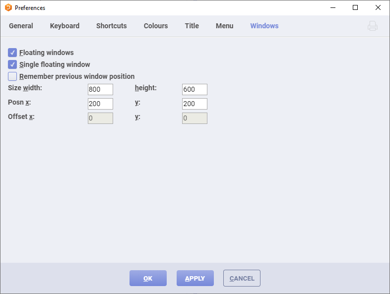
_images/RIDE_Configure_Floating_Windows.png

Fig. 5.5 Enable “floating” windows in RIDE.#

Working with floating windows has the added benefit of allowing you to have a stack of trace windows (as opposed to a single trace window), showing which functions call which other. This will be explored in Section 6.3.2.

5.1.2.2. A Text Editor; What For?#

Some dfns can be defined by a single expression and so are easy to define inside the session. We used this technique before to define a function named Average and here we do it again:

Average ← {(+/⍵)÷≢⍵}

However, as one defines more complex functions, it can become more complicated to define dfns in the session window.

For one, the ability to define multi-line dfns in the session was only made available with Dyalog 18.0. In these notebooks you can see that multi-line dfns are defined in cells that start with ]dinput:

]dinput
Average ← {
    (+/⍵)÷≢⍵
}

In the Windows interpreter an expression like the one above might result in a SYNTAX ERROR, as you type Average ← {, then hit Enter to change line, and then the interpreter tries to execute the line you entered, instead of allowing you to continue the definition of Average. To change this behaviour and allow for multi-line dfns, you can go to “Options” ⇨ “Configure…” ⇨ “Session” and check the experimental multi-line input box at the bottom. (If you are reading this and this book is old enough, the “experimental” multi-line input may no longer be experimental.)

If you are using RIDE and this capability is not ON by default, you can turn it ON by setting the DYALOG_LINEEDITOR_MODE environment variable to 1 in the connection menu, like demonstrated in Fig. 5.6.

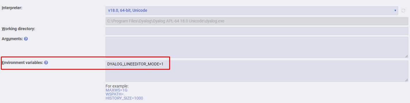
Fig. 5.6 Configuring RIDE to allow for multi-line input.#

Despite multi-line input, it is easier and more appropriate to edit multi-line dfns and tradfns in a suitable text editor. The built-in editors for the Windows interpreter and for RIDE are likely to be suitable for you, but other alternatives exist. You can find an enumeration of most of the available alternatives over at the APL Wiki. We will also cover this in more depth in the chapter about source code management.

5.2. Simple Dfns#

5.2.1. Definition#

Dfns are a set of statements enclosed by curly braces {}, so a simple dfn is typically created with the syntax Name ← { definition } where:

Name is the function name. It is followed by a definition, delimited by a pair of curly braces { and }. This definition may make use of one or two variables named ⍵ and ⍺, which represent the values to be processed. ⍵ and ⍺ are called arguments of the function;
⍵ (APL+w) is a generic symbol which represents the right argument of the function; and
⍺ (APL+a) is a generic symbol which represents the left argument if the function is dyadic.

Here is an example monadic dfn:

Average ← {(+/⍵)÷(≢⍵)}

And here are two more dyadic dfns, and an example showing how they can be used:

Plus ← {⍺ + ⍵}
Times ← {⍺ × ⍵}
3 Times 7 Plus 9

48

Notice the final statement above is strictly equivalent to

3 × 7 + 9

48

as the order of evaluation is the same.

The arguments ⍵ and ⍺ are read-only (they cannot be reassigned) and are limited in scope to only being visible within the function itself. The only exception to the “read-only rule” is when providing a default left argument to the dfn, which we’ll cover in Section 5.3.4.

The developer does not need to declare anything about the shape or internal representation of the arguments and the result. This information is automatically obtained from the arrays provided as its arguments. This is similar to the behaviour of dynamically typed programming languages, such as Python or Javascript. So, our functions can work on any arrays.

A scalar added to a matrix returns a matrix. No need to specify it:

12 Plus 2 3⍴⍳6

13 14 15 16 17 18

And a vector of integer numbers multiplied by a scalar fractional number returns a vector of fractional numbers:

7.3 Times 10 34 52 16

73 248.2 379.6 116.8

These simple dfns are well suited for pure calculations of straightforward array manipulation. For example, here is how we can calculate the hypotenuse of a right-angled triangle from the lengths of the two other sides:

Hypo ← {(+/⍵*2)*0.5}
Hypo 3 4

5

Hypo 12 5

13

5.2.2. Unnamed Dfns#

A dfn can be defined and then discarded immediately after it has been used, in which case it does not need a name. For example, the geometric mean of a set of n values is defined as the nth root of their product. The function can be defined and used inline like this:

{(×/⍵)*÷≢⍵} 6 8 4 11 9 14 7

7.8657

But because we didn’t assign it to a name, it was discarded after being used and can’t be used again. This kind of function is similar to inline, anonymous or lambda functions in other languages.

A special case is {}. This function does nothing, but placed at the left of an expression, it can be used to prevent the result of the expression from being displayed on the screen:

3 Plus 3

6

{} 3 Plus 3

5.2.3. Modifying The Code#

Single line dfns may be modified using the function editor, as will be explained in the next section. They can also be redefined entirely, as many times as necessary, as shown:

Magic ← {⍺+⍵}

Magic ← {⍺÷+/⍵}

Magic ← {(+/⍺)-(+/⍵)}

We defined Magic and then changed it twice. Only the most recent definition will survive.

Now we will delve into how to define and use more complex dfns. For this we will explore the built-in editor that comes with your interpreter and you will also learn some more syntax to empower your dfns.

5.3. More on Dfns#

The dfns we wrote in the previous section were very simple and consisted of a single statement. We will now use the text editor to define multi-line dfns.

5.3.1. Characteristics#

Generally, the opening and closing braces are placed alone on the first and last lines. This is not mandatory, it is just a convention;
dfns might be commented at will;
one can create as many variables as needed: they are automatically deemed to be local variables, which means they only exist while inside the dfn. Note that this is opposite to the default behaviour of tradfns, where all variables are global (cf. Section 5.3.3 and Section 5.6.2);
the arguments ⍵ and ⍺ retain the values passed to them as arguments and may not be changed. Any attempt to modify them causes a SYNTAX ERROR to be reported, except when defaulting the left argument (cf. Section 5.3.4);
as soon as an expression generates a result that is not assigned to a name or used in any other way, the function terminates, and the value of that expression is returned as the result of the function. If the function contains more lines they will not be executed (cf. Section 5.3.5); and
traditional control structures and branching cannot be used in dfns (cf. Section 5.5.1).

We will explore these characteristics in the following sections.

5.3.2. A Working Example#

As an example, let us see how we could define a function to calculate the harmonic mean of a vector of numbers. The harmonic mean of a vector is the inverse of the sum of the inverses of the numbers in the vector. This will become clearer when you see the code.

First of all, we must choose a name for our new function. We will choose to name it HarmonicMean.

Among the multiple ways of invoking the text editor, let us use a very simple one: type the command )ed followed by a space and the name of the function to create: )ed HarmonicMean.

Unless you already redefined the defaults, a mostly empty window should open to the right of the session. We include an example screenshot of such a window from the Windows interpreter, in Fig. 5.7:

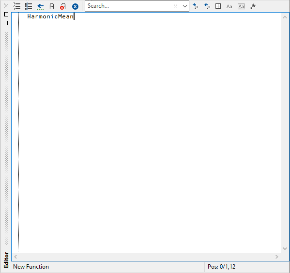
Fig. 5.7 The edit window opened by the command )ED HarmonicMean.#

Now that we have a window in which to define our dfn, we can go ahead and implement the harmonic mean. We shall split the process into a series of simple steps, as shown in Fig. 5.8: calculate the inverses, sum them, invert the sum.

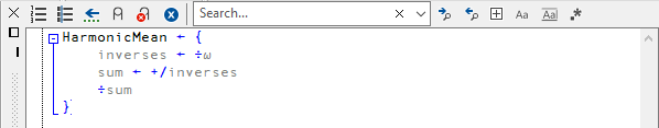
Fig. 5.8 The HarmonicMean function defined in the edit window.#

We also define it in this notebook:

]dinput
HarmonicMean ← {
    inverses ← ÷⍵
    sum ← +/inverses
    ÷sum
}

Now that we know how to compute the harmonic mean of a vector of numbers, we just have to fix it so that we can use it in our session. Fixing a function is somewhat analogous to compilation in other programming languages, but can also be seen as a sort of “File save” followed by an “import” in interpreted languages. There are many ways to fix a function:

Interpreter	Fix method
Windows interpreter	go to “File” ⇨ “Fix”
RIDE	right-click the edit window ⇨ “Fix”
both	press `Esc` (also closes the edit window)
both	define a custom keyboard shortcut

Following one of the appropriate methods should make the HarmonicMean function available for use in the session window. You can make sure it worked by simply typing in the name of the function and pressing Enter in the session:

HarmonicMean

{ inverses←÷⍵ sum←+/inverses ÷sum }

If instead of getting the source code of the function you get a VALUE ERROR, then the function wasn’t properly fixed.

Now that we can compute the harmonic mean of a vector of numbers, we can answer questions like the following:

“If I take 6 hours to paint a wall and you take 2 hours, how much time will we need to paint the wall if we do it together?”

This type of question can be answered by taking the harmonic mean of the individual times:

HarmonicMean 6 2

1.5

So the two of us would take one and a half hours to paint the whole wall.

Similarly, if we had further help from two people who could paint the whole wall in 4 and 5 hours, respectively, the four of us would need

times ← 6 2 4 5
⊢hours ← HarmonicMean times

0.895522

hours, or approximately

⌊60×hours

53

minutes.

After using your function for a bit you realise it is over-complicated, in the sense that it involves too many intermediate steps and you wish to get rid of those. If your edit window is still open, you can simply edit the function and fix it again. If the edit window was closed, you can type )ed HarmonicMean again or you can double-click the name HarmonicMean in the session. Both options will open the appropriate edit window.

After having done so, perhaps you rewrite your function to

]dinput
HarmonicMean ← {
    inverses ← ÷⍵
    ÷+/inverses
}

Then you fix it and use it again a couple of times:

HarmonicMean times

0.895522

HarmonicMean 4 3 2 1 0

DOMAIN ERROR: Divide by zero
HarmonicMean[1] inverses←÷⍵
                         ∧

But now it resulted in an error, and the error messages says HarmonicMean[1] inverses←÷⍵. This HarmonicMean[1] means the error was in line 1 of the HarmonicMean function. Right next to it, it also shows the part of the code that caused the error, but suppose you had a really long file, perhaps with multiple functions. How would you find the appropriate line in the first place?

Thankfully, both RIDE and the Windows interpreter have an option that can be set to display line numbers (cf. Fig. 5.9 and Fig. 5.10).

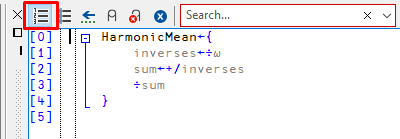
_images/Win_Editor_Toggle_Line_Numbers.png

Fig. 5.9 Option to toggle line numbers in RIDE (to the right) and the Windows interpreter (to the left).#

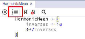
_images/RIDE_Editor_Toggle_Line_Numbers.png

Fig. 5.10 Option to toggle line numbers in RIDE, currently OFF.#

Different people like to comment their code in different ways, and naturally dfns can be commented. For illustrative purposes, consider the dfn that follows, which has comments before any statement, inline with some statements, between the statements and at the end of the dfn:

]dinput
HarmonicMean ← {
    ⍝ Monadic function to compute the harmonic mean of a vector
    inverses ← ÷⍵   ⍝ This inverts the numbers in the argument
    ⍝ and then
    ÷+/inverses     ⍝ we sum those inverses and return them.
    ⍝ Of course this will give an error if 0 is in the input argument.
}

The comments do not affect the behaviour of the function:

HarmonicMean times

0.895522

5.3.3. Local Variables#

Notice that our HarmonicMean function makes use of an intermediate variable, inverses. Let us check its value:

inverses

VALUE ERROR: Undefined name: inverses
      inverses
      ∧

We got a VALUE ERROR because inverses isn’t defined. It is a local variable, that is, a variable that lives within the dfn only while the dfn is being executed. As soon as we exit the dfn the variable stops existing.

The notion of local variable is opposed to the notion of global variable, which is a variable that lives in the session and thus can be accessed from anywhere. Useful global variables are functions themselves, because defining them globally means they can be used from within other functions.

As an example, we already defined the functions Average and HarmonicMean in the session. Let us now define a dfn named AMHM that checks empirically a mathematical theorem: that the arithmetic mean is always larger than or equal to the harmonic mean of a set of numbers:

]dinput
AMHM ← {
    am ← Average ⍵
    hm ← HarmonicMean ⍵
    am ≥ hm
}

AMHM ⍳6

1

AMHM times

1

Notice how the definition of AMHM uses both the Average and HarmonicMean dfns without defining them inside AMHM. This works because they were previously defined in the session.

For larger applications, proper source code management is needed and you should make sure the functions Average and HarmonicMean have been fixed when you use them inside AMHM, but that is a concern for later.

5.3.4. Default Left Argument#

It was mentioned above that the values of ⍺ and ⍵, the variables that represent the arguments to a dfn, cannot be assigned to. The only exception to this is when specifying a default left argument. This is relevant because a dyadic dfn can always be used monadically, as from the syntactic point of view its left argument ⍺ is always optional. If the left argument is not present it is possible to assign a default value to ⍺ by means of a normal assignment. If ⍺ is given a value because the dfn was called dyadically, such assignment is skipped.

Consider a function which calculates the nth root of a number, but which is normally used to calculate square roots. You can specify that the default value of the left argument (when omitted) is 2, as follows:

]dinput
Root ← {
    ⍺ ← 2
    ⍵*÷⍺
}

If we don’t specify the left argument of Root, it computes the square root. Root is thus said to be an ambivalent function, because it can be used both monadically and dyadically (cf. Section 5.10.3.3).

Root 625

25

But if we specify ⍺, then the ⍺ ← 2 assignment is skipped:

4 Root 625

5

Because the assignment with ⍺← is skipped entirely if ⍺ was provided, you should be careful with any side effects the expression to the right of ⍺← might produce. We illustrate this with the following (silly) example:

]dinput
Silly ← {
    a ← 1        ⍝ This assignment always happens
    ⍺ ← a ← 2    ⍝ Not executed if ⍺ already has a value
    a            ⍝ Return a
}

Silly 0

2

Because we didn’t provide a left argument, the ⍺ ← a ← 2 line is executed and a becomes 2.

On the other hand, if we provide a left argument the ⍺ ← a ← 2 line is skipped and a remains 1:

0 Silly 0

1

As for ⍵, attempting to assign to ⍵ makes no sense: a dfn is always called monadically or dyadically, so the right argument is always present. Here’s a function that computes the square root of ⍵, except that first it tries to assign 10 to ⍵:

]dinput
RootOf10 ← {
    ⍵ ← 10
    ⍵*0.5
}

Simply typing the name of the function shows its code:

RootOf10

{ ⍵←10 ⍵*0.5 }

And calling it monadically raises an error:

RootOf10 5

SYNTAX ERROR
RootOf10[1] ⍵←10
             ∧

5.3.5. Returning the Result#

We mentioned above that a dfn executes its statements until the first statement that does not assign its value. Here is a curious dfn with 4 statements:

]dinput
Count ← {
    1
    2
    3
    10÷0
}

Notice that all four statements are simple. If we run Count, what will the result be?

Count 73

1

The result we get is 1 because the first statement evaluates to 1 (obviously) and then we do nothing with it, so that is what the dfn returns. It doesn’t matter what we wrote afterwards and it doesn’t even matter that the very last statement would give a DOMAIN ERROR.

These superfluous statements should be avoided, as they will sooner or later cause unnecessary confusion.

As a basic debugging tool, it is possible to modify statements to display intermediate results:

]dinput
Count ← {
    ⎕←1
    ⎕←2
    ⎕←3
    10÷0
}

Count 73

1
2
3
DOMAIN ERROR: Divide by zero
Count[4] 10÷0
           ∧

Be careful: by using ⎕← to display intermediate results, suddenly we are doing something with the superfluous statements and they are all being executed (we even reached the error statement).

And even if we remove the statement that gives an error, the function will still return something other than the original 1:

]dinput
Count ← {
    ⎕←1
    ⎕←2
    3
}

Count 73

1 2 3

Now the function returned 3 instead of 1! So always be careful with which statement is actually giving the final result and avoid any extraneous statements.

5.4. Exercises on Dfns#

You are ready to solve simple problems. We strongly recommend that you try to solve all the following exercises before you continue further in this chapter. Many of the exercises are followed by some examples you can use to check your work.

Exercise 5.1

Write a dyadic function Extract which returns the first ⍺ items of any given vector ⍵.

Here are some examples:

3 Extract 45 86 31 20 75 62 18

45 86 31

45 86 31 ≡ 3 Extract 45 86 31 20 75 62 18

1

6 Extract 'can you do it?'

can yo

'can yo' ≡ 6 Extract 'can you do it?'

1

Exercise 5.2

Write a dyadic function Ignore which ignores the first ⍺ items of any given vector ⍵ and only returns the remainder.

3 Ignore 45 86 31 20 75 62 18

20 75 62 18

20 75 62 18 ≡ 3 Ignore 45 86 31 20 75 62 18

1

6 Ignore 'can you do it?'

u do it?

'u do it?' ≡ 6 Ignore 'can you do it?'

1

Exercise 5.3

Write a monadic function Reverse which returns the items of a vector in reverse order.

Reverse 'snoitalutargnoc'

congratulations

Reverse '!ti did uoY'

You did it!

Exercise 5.4

Write a monadic function Totalise which appends row and column totals to a numeric matrix.

⊢mat ← 3 4⍴75 14 86 20 31 16 40 51 22 64 31 28

75 14 86 20 31 16 40 51 22 64 31 28

⊢totMat ← Totalise mat

75 14 86 20 195 31 16 40 51 138 22 64 31 28 145 128 94 157 99 478

Notice that mat occupies the upper left corner of totMat:

totMat ∊ mat

1 1 1 1 0 1 1 1 1 0 1 1 1 1 0 0 0 0 0 0

Exercise 5.5

Write a monadic function Lengths which returns the lengths of the words contained in a text vector.

Lengths 'This seems to be a good solution'

4 5 2 2 1 4 8

4 5 2 2 1 4 8 ≡ Lengths 'This seems to be a good solution'

1

Exercise 5.6

Write a dyadic function To which produces the series of integer values between the limits given by its two arguments.

17 To 29

17 18 19 20 21 22 23 24 25 26 27 28 29

Exercise 5.7

Develop a monadic function Frame which puts a frame around a text matrix. For the first version, just concatenate minus signs above and under the matrix, and vertical bars down both sides. Then, update the function to replace the four corners by four + signs.

⊢towns ← 6 10⍴'Canberra  Paris     WashingtonMoscow    Martigues Mexico    '

Canberra Paris Washington Moscow Martigues Mexico

Frame towns

Finally, you can improve the appearance of the result by changing the function to use line-drawing symbols. You enter line-drawing symbols by using ⎕UCS, a system function that converts characters to integers and vice-versa:

⎕UCS 9472 9474

─│

⎕UCS 9484 9488 9492 9496

┌┐└┘

Correspondingly, applying ⎕UCS to those characters yields the original integers:

⎕UCS '─│┌┐└┘'

9472 9474 9484 9488 9492 9496

After improving your function, the result should look like this:

Frame towns

┌──────────┐ │Canberra │ │Paris │ │Washington│ │Moscow │ │Martigues │ │Mexico │ └──────────┘

Exercise 5.8

It is very likely that the function you wrote for the previous exercise works on matrices but not on vectors. Can you make it work on both?

Frame 'We are not out of the wood'

┌──────────────────────────┐ │We are not out of the wood│ └──────────────────────────┘

Exercise 5.9

Write a function Switch which replaces a given letter by another one in a text vector. The letter to replace is given first; the replacing letter is given second.

'tc' Switch 'A bird in the hand is worth two in the bush'

A bird in che hand is worch cwo in che bush

Exercise 5.10

Modify the previous function so that it commutes the two letters.

'ei' Swap 'A bird in the hand is worth two in the bush'

A berd en thi hand es worth two en thi bush

5.5. Dfns in Depth#

In this section we will cover a couple of more advanced subtleties about dfns, and then we will move on to learn about tradfns.

5.5.1. Guards#

Previously we said that control structures cannot be used in dfns. However, it is possible to have a dfn conditionally calculate a result, by using a guard.

A guard is any expression which generates a one-item Boolean result, followed by a colon.

The expression placed to the right of a guard is executed only if the guard is true. In a dfn, this looks like guard: expr and works similarly to a

if (guard) {
    return expr;
}

of some popular programming languages.

For example, this function will give a result equal to 'Positive', 'Zero' or 'Negative' if the argument ⍵ is respectively greater than, equal to, or smaller than zero:

]dinput
Sign ← {
    ⍵>0: 'Positive'
    ⍵=0: 'Zero'
    'Negative'
}

Sign 3

Positive

Sign ¯3.6

Negative

Sign 0

Zero

5.5.2. Shy Result#

Dfns can be written in such a way that they return a shy result. A shy result is a result which is returned, but not displayed by default.

Consider a function which deletes a file from disk and returns a result equal to 1 (file deleted) or 0 (file not found). Usually, one doesn’t care if the file did not exist, so the result is not needed. But sometimes it may be important to check whether the file really existed and has been removed. So, sometimes a result is useless and sometimes it is useful… this is the reason why shy results have been invented.

In a dfn, a shy result happens when the last expression that is evaluated is assigned to a (local) name, as opposed to just leaving the result of the expression unassigned. For this to happen, one has to be careful to leave the closing curly brace } next to that final statement, instead of having } alone in a new line.

Here is the function above, written without guards and with a shy result:

Sign ← { s ← (3 8⍴'NegativeZero    Positive')[2+×⍵;] }

Sign 3

Sign ¯3.6

⎕← Sign 0

Zero

Notice what happens if we were to format Sign as we have formatted previous dfns:

]dinput
Sign ← {
    s ← (3 8⍴'NegativeZero    Positive')[2+×⍵;]
}

Sign 3

Sign ¯3.6

⎕← Sign 0

VALUE ERROR: No result was provided when the context expected one
      ⎕←Sign 0
        ∧

The VALUE ERROR we get above is a very subtle error. Because the s ← ... statement is an assignment, when executing the Sign dfn the interpreter goes on to execute the expression on the next line, but the next line has no expression and so the interpreter raises a VALUE ERROR. If we want to have a shy result on a multi-line dfn, we must have the final curly brace on the same line as the final statement.

5.5.3. Lexical Scoping#

Lexical scoping (also referred to as static scoping) is the mechanism that turns local and global variables into relative notions that depend on the context in which dfns were defined: dfns usually have access to global variables, but the variables that are “global” depend on where the dfn was written.

As a purely illustrative example, consider the function defined below:

]dinput
MultiplyBy10← {
    v ← 10            ⍝ define some variable
    TimesV ← {v×⍵}    ⍝ multiply something with v
    TimesV ⍵
}

MultiplyBy10 5

50

MultiplyBy10 10

100

Notice how the MultiplyBy10 function takes your input and gives it to the TimesV function, which is defined as a function that “takes its input (⍵) and multiplies it with v”. But what is v? We do not give a value to v inside TimesV, so when APL encounters the expression v×⍵ it looks at its surroundings for the meaning of v. Because v was defined in the enclosing dfn as v ← 10, that is the value that is used.

Consider now a similar example, but with more occurrences of the variable v:

v ← 100          ⍝ (1)

]dinput
MultiplyBy10 ← {
    GiveMeV ← {
        v
    }
    ⎕← v         ⍝ (3)
    ⎕← GiveMeV 1 ⍝ (4)
    v ← 10       ⍝ (5)
    ⎕← v         ⍝ (6)
    ⎕← GiveMeV 1 ⍝ (7)
    v ← 10×⍵     ⍝ (8)
    v
}

⎕← v             ⍝ (2)
MultiplyBy10 3
⎕← v             ⍝ (9)

100

100 100 10 10 30

100

Let us go over the assignments and the outputs of the code above:

we start by defining the variable v in our session and we set it to 100 (1);
we then define a function named MultiplyBy10 which happens to contain another dfn inside it;
then we print the value of the session variable v and we see its value is 100 (2);
then we call the dfn MultiplyBy10 with argument 3 and
- we define a new dfn named GiveMeV;
- we print the value of v (3). MultiplyBy10 doesn’t know what v is and so it looks for it in the session and finds a v whose value is 100, because of (1);
- we then call the function GiveMeV which simply returns v and we print it (4). GiveMeV doesn’t know what v is, so it asks MultiplyBy10, which in turns asks the session, which knows of a v whose value is 100, because of (1);
- we then define v to be 10 inside of MultiplyBy10 (5), making MultiplyBy10 aware of a variable v;
- then we print v inside MultiplyBy10 (6), which is 10 because we just defined it as such;
- then we call GiveMeV again and we print its result (7). GiveMeV doesn’t know what v is, so it asks MultiplyBy10, that now knows what v is: it is 10 because of (5);
- and we finish executing the MultiplyBy10 dfn by assigning 30 to v (8), which we then return from the dfn;
we leave the MultiplyBy10 dfn call and 30 gets printed because that was the result of the dfn call;
finally we print v once more, and the session knows v is 100, so that is what we print (9).

That might look confusing, but I assure you it makes a lot of sense. Just go through the code calmly and make sure you understand what each part does separately. Then, simulate the execution of the code with some pen and paper and write down what you think should get printed at each step. Then read the explanation above and compare it to what you thought was supposed to happen. You will get used to lexical scoping in no time.

Lexical scoping can reveal itself to be extremely useful in languages where functions can return other functions, which is not the case with APL. Even so, lexical scoping will prove to be helpful later down the road: imagine a large(r) function inside which we define a small utility dfn to use with an operator, but we want the dfn to make use of things we have already computed inside the outer function. Lexical scoping kicks in at that point, allowing the inner dfn to access everything the outer function already computed.

This concludes the more advanced topics on dfns. If you are used to programming in other programming languages that follow paradigms other than the array-oriented one, dfns may look very limited in their lack of conventional control structures and looping structures. As it turns out, in writing good array-oriented programs you can usually do away without these. What is more, the power of many of the built-in operators you will learn about in a future chapter will cover that gap in a very suitable way.

5.6. Tradfns#

Tradfns, which were previously referred to as procedural functions, are mainly used for complex calculations involving many variables, interactions with a user, file input/output of data, etc. They look much like functions or programs in more traditional programming languages.

Tradfn is short for “traditional function”, because in the beginning APL did not have support for dfns. Hence, when dfns were a novelty, tradfns were the traditional functions that had been around for a while.

5.6.1. A First Example#

Tradfns are composed of a header and one or more statements (function lines), so invoking a text editor to enter these lines of text will make your life easier.

As an example, let us see how we could define the HarmonicMean from before as a tradfn. Let us call it TradHarmonicMean, for traditional harmonic mean.

Let us open the editor with )ed TradHarmonicMean and outright define our function:

∇ mean ← TradHarmonicMean argVector
    inverses ← ÷argVector
    mean ← ÷+/inverses
∇

Now I will break it down for you:

The function is delimited by a pair of ∇ symbols. This special symbol is named del in English, or carrot (because of its shape) in some French-speaking countries. You can type a del with APL+g. In Jupyter notebooks and in the session, those are mandatory. If you define the tradfn in the text editor, you can omit them (cf. Fig. 5.11);

The first line of the tradfn is the header and tells APL that:

the tradfn is going to be called TradHarmonicMean;
it expects a right argument which will be named argVector; and
it will return the value we store in the variable named mean.

The subsequent lines have the statements of the function itself and, in particular, the final line in which we perform the mean ← ... assignment is where we establish the result that will be returned by the tradfn.

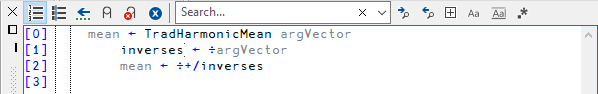
Fig. 5.11 A tradfn defined in the editor and without delimiting Del characters.#

The function is now available for use:

TradHarmonicMean 2 6

1.5

5.6.2. The Default Isn’t Local#

Just like when we defined HarmonicMean as our first dfn, our tradfn uses a temporary variable called inverses. Let us check its value:

inverses

0.5 0.166667

When we did the same check in Section 5.3.3, we couldn’t access the value of inverses because it was not defined in the session, it was a variable that was local to the dfn. Clearly, this works differently in tradfns.

If you were paying attention, you will have noticed that in Fig. 5.11 there’s two colours being used (the actual colours might differ between the Windows IDE and RIDE, and you might also have changed your colour scheme to something else):

black for the names TradHarmonicMean and inverses; and
grey for the names argVector and mean.

So what do the colours mean?

The names in black are the variables that are global, variables that remain in the workspace after they have been assigned values during execution of the function. These names can refer to existing variables - intentionally or not - and may produce undesirable side effects.

The names in grey are temporary variable names used during function execution. Once execution is complete, these temporary variables are destroyed. Right before that, the tradfn returns the value of the return variable - mean in our example - and then discards its name.

That means neither argVector nor mean should be available after execution of the tradfn ends:

mean

VALUE ERROR: Undefined name: mean
      mean
      ∧

argVector

VALUE ERROR: Undefined name: argVector
      argVector
      ∧

Because inverses is coloured in black, we can see it can interfere with the variables in our workspace:

inverses ← 'The inverses are calculated by use of monadic ÷'
TradHarmonicMean 1 2 3 4

0.48

And suddenly inverses is no longer what you defined:

inverses

1 0.5 0.333333 0.25

All the variables created during execution of the tradfn that are not referenced in the header are considered to be global variables. To avoid any unpredictable side effects, it is recommended that you declare as local all the variables used by a function. This is done by specifying their names in the header, each prefixed by a semi-colon, as shown in this new definition of TradHarmonicMean:

∇ mean ← TradHarmonicMean argVector; inverses
    inverses ← ÷argVector
    mean ← ÷+/inverses
∇

inverses ← 'The inverses are calculated by use of monadic ÷'
TradHarmonicMean 1 2 3 4

0.48

inverses

The inverses are calculated by use of monadic ÷

As we can see, inverses is now treated as a local variable.

Rules

All the names referenced in the header of a function (including its result and arguments) are local to the function. They will exist only during the execution of the function.
Operations made on local variables do not affect global variables having the same names.
Global and local are relative notions: when a tradfn calls another sub function, variables local to the calling function are global for the called function. This will be further explored in Section 5.6.5.
All the variables used in a tradfn should preferably be declared local, unless you specifically intend otherwise.

5.6.3. Defining Sub-Functions#

As we have seen, dfns can be defined inside other dfns. Similarly, dfns can be defined inside tradfns and used right away. The precautions mentioned above, that need to be taken with respect to global versus local variables, still apply. In short, do not forget to localise the name of a temporary dfn unless you really mean for it to become global.

5.6.4. A Second Example#

You may remember from previous chapters our two matrices forecast and actual, representing sales of 4 products over 6 months:

⎕RL ← 73
⊢forecast ← 10×?4 6⍴55

90 160 420 500 20 30 110 450 170 370 290 360 340 190 320 120 510 370 150 460 240 520 490 280

⎕RL ← 73
⊢actual ← forecast + ¯10+?4 6⍴20

89 166 420 508 12 23 111 453 177 365 284 352 349 192 329 115 515 374 160 467 234 519 485 283

It would be nice to interlace the columns of those two matrices to make it easier to compare forecast and actual sales for the same month. Furthermore, because this might be useful for other pairs of matrices, let’s create a general function to do the job; let’s call it Interlace.

The result we would like to obtain is schematised in the table below, with f being shorthand for forecast and a being shorthand for actual:

`f[;1]`	`a[;1]`	`f[;2]`	`a[;2]`	`f[;3]`	`a[;3]`	`f[;4]`	`a[;4]`	`f[;5]`	`a[;5]`	`f[;6]`	`a[;6]`
90	89	160	166	420	420	500	508	20	12	30	23
110	111	450	453	170	177	370	365	290	284	360	352
340	349	190	192	320	329	120	115	510	515	370	374
150	160	460	467	240	234	520	519	490	485	280	283

The first thing you must decide is how this function will be used:

will you pass both matrices on right: Interlace forecast actual; or
one on the left and one on the right: forecast Interlace actual?

Both solutions are valid; it is only a question of personal taste and ease of use. Our first tradfn was monadic so let us make this one dyadic.

Having decided on the calling syntax, we just have to know how the header of a dyadic tradfn looks like. If we call r to the result and x and y to the left and right arguments, respectively, then the tradfn header is

∇ r ← x Interlace y
∇

which may then be updated to include local variables.

The names x, y and r do not matter to the APL system. Replacing x and y with a and b or left and right would be perfectly valid and obviously easier to recall than if we replaced them with potatoes and ocarina. However, you should pick names which help you remember what the function is doing. For example, in a general-purpose function like this, you should probably avoid using too specific names like forecast and actual: that would imply that this function only works on arrays containing forecast and actual data. Such names might also confuse the distinction between local and global names.

Now that the header is set, how shall we interlace our two matrices? Have a go at it, if you fancy.

We suggest the following steps:

calculate the size of the result r. It will be a matrix with as many rows as x and y, but twice as many columns;
create r filled with zeroes;
calculate the indices of its even columns;
fill the even columns with y;
calculate the indices of its odd columns and fill them with x.

The final function could be written as follows. Do not forget to localise your variables.

∇ r ← x Interlace y; size; even
    size ← 1 2×⍴x
    r ← size⍴0
    even ← 2×⍳(⍴x)[2]
    r[;even] ← y
    r[;even-1] ← x
∇

We can now apply the function to any pair of variables, provided they have the same size:

forecast Interlace actual

90 89 160 166 420 420 500 508 20 12 30 23 110 111 450 453 170 177 370 365 290 284 360 352 340 349 190 192 320 329 120 115 510 515 370 374 150 160 460 467 240 234 520 519 490 485 280 283

(2 3⍴⍳6) Interlace (2 3⍴¯5 ¯7 ¯1 ¯2 ¯8 ¯9)

1 ¯5 2 ¯7 3 ¯1 4 ¯2 5 ¯8 6 ¯9

5.6.4.1. Another Possible Syntax#

If you had decided instead to make the function monadic, it could look very similar to the one above. We just changed the header a bit and added a new statement at the beginning:

∇ r ← Interlace couple; x; y; size; even
    (x y) ← couple
    size ← 1 2×⍴x
    r ← size⍴0
    even ← 2×⍳(⍴x)[2]
    r[;even] ← y
    r[;even-1] ← x
∇

Interlace forecast actual

90 89 160 166 420 420 500 508 20 12 30 23 110 111 450 453 170 177 370 365 290 284 360 352 340 349 190 192 320 329 120 115 510 515 370 374 150 160 460 467 240 234 520 519 490 485 280 283

5.6.5. Dynamic Scoping#

Dynamic scoping (as opposed to static scoping, as seen in Section 5.5.3) is the scoping mechanism that tradfns use: when a tradfn calls another tradfn, the callee can see the caller’s local variables, even if the callee was defined outside of the caller.

To explore what this means, consider the following tradfns. Do not worry about their arguments and return values as they are not meaningful. What matters are the assignments to a and b and the prints.

∇ r ← PrintAB y
    ⎕← a
    ⎕← b
    r ← 0
∇

∇ r ← SetAThenPrint y; a
    a ← 1
    r ← PrintAB y
∇

∇ r ← SetBThenPrint y; b
    b ← 2
    r ← PrintAB y
∇

and let us define global variables a and b with character values:

a ← 'a'
b ← 'b'

Now let us call SetAThenPrint. Before looking at the code that follows, what do you expect to be printed?

SetAThenPrint 0

1 b 0

Did it match your expectations? Can you now guess what will happen if we execute SetBThenPrint?

SetBThenPrint 0

a 2 0

Notice how PrintAB was defined as a standalone tradfn which prints two variables. Because a and b are never defined inside PrintAB, surely PrintAB will be printing global values. Then, depending on what function called PrintAB, either a or b are taken from the context of the enclosing calling function.

Let us try to define the same functions but with dfns:

]dinput
PrintCD ← {
    ⎕← c
    ⎕← d
    0
}

]dinput
SetCThenPrint ← {
    c ← 3
    PrintCD ⍵
}

]dinput
SetDThenPrint ← {
    d ← 4
    PrintCD ⍵
}

c ← 'c'
d ← 'd'

What will happen if we call SetCThenPrint?

SetCThenPrint 0

c d 0

Even though SetCThenPrint modified the value of c to be 3, the PrintCD function was defined in the workspace, and hence its lexical scoping tells it to look for c among its own variables, and among the global variables in the workspace. PrintCD does not have access to the local variables of the dfn that called it.

That is why, if we call SetDThenPrint, we get the exact same output:

SetDThenPrint 0

c d 0

Perhaps the difference between dynamic and lexical scoping becomes even more clear if we consider yet another family of tradfns:

∇ r ← PrintE y
    ⎕← e
    r ← 0
∇

Notice that if you call PrintE right now it will cause an error, because there is no variable e defined anywhere:

VALUE ERROR: Undefined name: e
      e
      ∧

PrintE 0

VALUE ERROR: Undefined name: e
PrintE[1] ⎕←e
            ∧

Now let us define a tradfn that makes use of a local variable e:

∇ r ← SetLocalE y; e
    e ← 5
    r ← PrintE y
∇

If we call SetLocalE, e will be defined inside SetLocalE and then, when PrintE gets called, the dynamic scoping will make e visible as a global variable:

SetLocalE 0

5 0

After SetLocalE is executed, our workspace still has no variable e:

VALUE ERROR: Undefined name: e
      e
      ∧

Scoping can become messy quickly, and that is why it is recommended that you always provide the information your functions need as arguments, and return the results explicitly instead of relying on modifying some global variable(s). In Section 5.16.2 we will see this can become even more confusing when you start having dfns calling tradfns and tradfns calling dfns.

5.7. Flow Control in Tradfns#

5.7.1. Overview#

Apart from extremely simple calculations, most programs rely on certain statements being executed only if a given condition is satisfied (conditional execution) or on a set of statements being executed again and again, until a given limit is reached (looping). The APL language offers a special set of syntactic elements to control the flow of statements inside tradfns.

In the very first versions of APL, the only way to implement conditional execution and looping was to use the symbol → (the branch arrow, typed with APL+]). This was used to jump from one statement to another, skipping over other statements (conditional execution) or jumping back to repeat a set of statements again (looping). The branch arrow is equivalent to the GOTO statement in other languages. Contemporary versions of APL include a special set of keywords which offer a much more flexible, easy to use and easy to read way to control the flow of execution. They are also very similar to those used in most other languages. These are known as control structures.

We shall begin by using control structures and then introduce you later to the old way of programming (using →), only because you may come across it in some existing programs and it will be helpful to be able to read those.

Control structures are blocks of statements which begin and end with special keywords. These keywords are all prefixed with a colon, like :If or :Repeat. This prevents the names of your variables to clash with these keywords.

The keywords can be typed in lower or upper case, but Dyalog APL will always store and display them using a fixed spelling convention commonly known as CamelCase or, more specifically, PascalCase. Following this convention, a keyword has an upper case first letter and the following letters in lower case. Composite keywords like “EndIf” and “GoTo” capitalise the first letter of each word.

Opening keywords are used to begin the conditional execution or repeated execution of a block of statements. Usually (but not always), the block is ended by a corresponding keyword that starts with :End.

The sets of opening/closing keywords are shown below:

Opening	Closing
`:If`	`:EndIf`
`:For`	`:EndFor`
`:Select`	`:EndSelect`
`:Repeat`	`:Until`
	`:EndRepeat`
`:While`	`:EndWhile`
	`:Until`
`:Trap`	`:EndTrap`
`:With`	`:EndWith`
`:Hold`	`:EndHold`

The primary keywords shown above can be complemented by additional keywords which qualify more precisely what is to be done:

:Else
:ElseIf
:AndIf
:OrIf
:Case
:CaseList
:Until

And finally, some keywords may be used to conditionally alter the flow of execution within a control structure.

The following keywords will not be studied in this chapter:

:Trap... :EndTrap concerns event processing and will be seen in the chapter “Event Handling”;
:With... :EndWith concerns the GUI interface and namespaces and will be covered in the chapter on GUIs and in the chapter on namespaces;
:Hold... :EndHold concerns multi threading.

5.7.2. Conditional Execution#

5.7.2.1. Simple Conditions (`:If`/`:EndIf`)#

The clauses :If and :EndIf delimit a block of statements (Block 1 in Fig. 5.12), which will be executed only if the condition specified by the :If clause is satisfied.

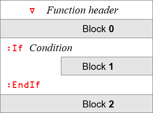
Fig. 5.12 A diagram with the usage of :If... :EndIf.#

Here is the explanation of what happens inside the function of the diagram Fig. 5.12:

if present, Block 0 will always be executed, as will Block 2;
Condition is any expression whose result is a Boolean scalar or one-item array; for example, code∊list, price>100 or values∧.=0; and
Block 1 will be executed if Condition is satisfied.

Example

Our keyboard has been damaged: we can no longer use the absolute value key. Perhaps a tradfn could replace it? Try writing a tradfn using an :If clause.

Here is a possible solution:

∇ y ← AbsVal y
    :If y < 0
        y ← -y
    :EndIf
∇

AbsVal 1

1

AbsVal ¯3.4

3.4

If the argument is positive (or zero), the function does nothing and just returns the argument it received. If the argument is negative, it returns the corresponding positive value.

5.7.2.2. Alternative Processing (`:If`/`:Else`/`:EndIf`)#

In the previous example if Condition is satisfied, Block 1 is executed; otherwise nothing is done. But sometimes we would like to execute one set of statements (Block 1) if Condition is satisfied or an alternative one (Block 2) if it is not.

For this, we use the additional keyword :Else as shown in Fig. 5.13:

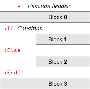
Fig. 5.13 A diagram with the usage of :If... :Else... :EndIf.#

Blocks 0 and 3 will always be executed, if present. Block 1 will be executed if Condition is satisfied and Block 2 will be executed if Condition is not satisfied. Notice this means that exactly one of the two blocks gets executed. Never both, and never none.

Example

Let us try to find the real roots of the quadratic equation \(ax^2 + bx + c = 0\), given the values of \(a\), \(b\) and \(c\). If the quantity \(\Delta = b^2 - 4ac\) is negative, it is known that the two solutions of this equation are complex numbers. \(\Delta\) is commonly referred to as the discriminant of the equation.

We can write a tradfn that computes the two roots by means of the quadratic formula, except that it issues an error message if there are no real roots. We will use an :If... :Else... :EndIf clause for this:

∇ r ← QuadRoot abc; a; b; c; delta
    (a b c) ← abc
    delta ← (b*2)-4×a×c
    :If delta≥0
        r ← (-b)+1 ¯1×delta*0.5
        r ← r÷2×a
    :Else
        r ← 'No roots'
    :EndIf
∇

QuadRoot ¯2 7 15

¯1.5 5

QuadRoot 1 1 1

No roots

5.7.2.3. Composite Conditions (`:OrIf`/`:AndIf`)#

Multiple conditions can be combined using the Boolean functions or and and.

Consider the diagram Fig. 5.14:

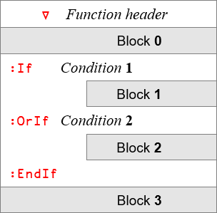
Fig. 5.14 A diagram with the usage of :OrIf.#

If present, Block 0 and Block 3 will always be executed. Block 1 and Condition 2 are only executed if Condition 1 is not satisfied. Block 2 is executed if Condition 1 OR Condition 2 is satisfied.

In many cases, the same result could be obtained by a more traditional APL approach using ∨: :If (Condition 1) ∨ (Condition 2).

However, suppose that Block 1 and/or Condition 2 need a lot of computing time.

The traditional APL solution will always evaluate both Condition 1 and Condition 2, combine the results, and decide what to do.
With the “:OrIf” technique, if Condition 1 is satisfied, Block 2 will be immediately executed, and neither Block 1 nor Condition 2 will be evaluated. This may sometimes save a lot of processing time.

Using the :OrIf clause will thus enable what is usually referred to as short-circuiting in other programming languages.

Note that the optional Block 1 may be useful to prepare the variables to be referenced in Condition 2, but can also be omitted.

We have a similar structure with the :AndIf clause, as seen in Fig. 5.15:

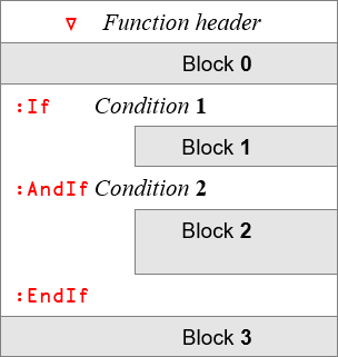
Fig. 5.15 A diagram with the usage of :AndIf.#

Again, Block 0 and Block 3 will always be executed. Block 1 is optional and will only be executed if Condition 1 is satisfied. Likewise, Condition 2 will be executed only if Condition 1 is satisfied. Finally, Block 2 is executed if both Condition 1 AND Condition 2 are satisfied.

Rule

For :OrIf and :AndIf, Block 1 and Condition 2 are only executed if the result of Condition 1 is not enough to determine the result of the Boolean operation combining conditions 1 and 2.

In many cases, the same result could be obtained by a more traditional APL approach using ∧: :If (Condition 1) ∧ (Condition 2).

However, it may be that Condition 2 cannot be evaluated if Condition 1 is not satisfied. For example, we want to execute Block 2 if the variable var exists and is smaller than the argument arg. It is obvious that var<arg cannot be evaluated if the variable var does not even exist. The two conditions must be evaluated separately:

∇ r ← CheckVar arg
    r ← 0
    :If 2=⎕NC'var'
        ⎕← 'var exists'
    :AndIf var<arg
        ⎕← 'var is smaller than arg'
        r ← 1
    :EndIf
∇

Notice that var doesn’t exist as a variable in our workspace:

var

VALUE ERROR: Undefined name: var
      var
      ∧

Hence CheckVar should do nothing and return 0:

CheckVar 1000

0

If Condition 1 is not satisfied neither Block 1 nor Condition 2 are executed. This may also save some computing time in more complex tradfns.

Now we set var to some value and we can then check it:

var ← 500

CheckVar 1000

var exists var is smaller than arg 1

CheckVar 100

var exists 0

Note that you may not combine :OrIf and :AndIf within the same control structure. The following code will generate a SYNTAX ERROR:

∇ surface ← BadSyntaxTradfn args; width; length; height
    (width length height) ← args
    :If width<20
    :AndIf length<100
    :OrIf height<5
        surface ← 0
    :Else
        surface ← width×length
    :EndIf
∇

BadSyntaxTradfn 5 5 5

SYNTAX ERROR
BadSyntaxTradfn[2] :If width<20
                            ∧

5.7.2.4. Cascading Conditions (`:ElseIf`/`:Else`)#

Sometimes, if the first condition is not satisfied, perhaps a second or a third one will be. In each case, a different set of statements will be executed. This type of logic may be controlled by one or more “:ElseIf” clauses. And if none of these conditions are satisfied, perhaps another block of statements is to be executed; this may be controlled by a final “:Else”, as we have seen earlier.

Depending on the problem, “:Else” may be present or not. If there is no “:Else” clause and no condition has been satisfied, nothing will be executed inside the :If block.

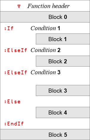
Fig. 5.16 A diagram with multiple usages of :ElseIf clauses.#

By now, you should be able to tell by yourself that Block 0 and Block 5 in Fig. 5.16, if present, will always be executed.

For the conditions and the remaining blocks, a simple rule applies:

Rule

Using Fig. 5.16 as reference for the rule examples:

the conditions are executed in turn, until one of them is satisfied. When one condition is satisfied, its corresponding block is executed. For example, if Condition 1 is not satisfied and Condition 2 is satisfied, then Block 2 is executed;

as soon as one condition is satisfied and its block is executed, all other conditions and blocks inside the :If... :EndIf control structure are ignored. For example, if Condition 2 is the first condition to be satisfied, then Condition 3 is not executed (even if Condition 3 would be satisfied), as neither are Block 3 nor Block 4; and

if none of the conditions is satisfied and an :Else clause is present, then its corresponding block is executed. For example, if conditions 1 to 3 are not satisfied, then Block 4 is satisfied.

Hence, all conditional blocks (blocks 1 to 4) are mutually exclusive.

For example, suppose that the first condition is var<100 and the second is var<200.

If var happens to be equal to 33, it is both smaller than 100 and 200, but only the block of statements attached to var<100 will be executed:

∇ r ← VarLevels var
    :If var<100
        ⎕← 'var is < than 100'
        r ← 100
    :ElseIf var<200
        ⎕← 'var is < than 200'
        r ← 200
    :Else
        ⎕← 'var is too big'
        r ← var
    :EndIf
∇

VarLevels 33

var is < than 100 100

VarLevels 133

var is < than 200 200

VarLevels 350

var is too big 350

5.7.2.5. Alternative Solutions#

Now you know how to use control structures to write conditional expressions. However, this does not mean that you always have to or should use control structures. The richness of the APL language often makes it more convenient to express condition calculations using a more mathematical approach.

For example, suppose that you need to comment on the result of a football or rugby match by displaying “Won”, “Draw” or “Lost”, depending on the scores of the two teams. Here are two solutions:

∇ r ← x Comment y
    :If x>y
        r ← 'Won'
    :ElseIf x=y
        r ← 'Draw'
    :Else
        r ← 'Lost'
    :EndIf
∇

2 Comment 1

Won

2 Comment 2

Draw

0 Comment 3

Lost

∇ r ← x Comment y
    which ← 2+×x-y
    r ← (3 4⍴'LostDrawWon ')[which;]
∇

2 Comment 1

Won

2 Comment 2

Draw

0 Comment 3

Lost

Which solution you prefer is probably a matter of taste and previous experience, both yours and of whoever is to read and maintain the programs you write. Notice that only the second solution is suitable for a dfn.

5.7.3. Disparate Conditions#

5.7.3.1. Clauses (`:Select`/`:Case`/`:CaseList`)#

Sometimes it is necessary to execute completely different sets of statements, depending on the value of a specific control expression, hereafter called the control value.

To achieve this, we use “:Select”, with additional “:Case” or “:CaseList” clauses.

The sequence begins with :Select followed by the control expression.

It is then followed by any number of blocks, each of which will be executed if the control value is equal to one of the values specified in the corresponding clause:

:Case for a single value.
:CaseList for a list of possible values.

The sequence ends with :EndSelect.

You can have as many :Case or :CaseList clauses as you need and in any order.

If the control value is not equal to any of the specified values, nothing is executed, unless there is one final :Else clause.

Like with :If... :ElseIf... :Else, the blocks are mutually exclusive. The :Case statements are examined from the top and once a match is found and the corresponding block of statements has been executed, execution will continue with the first line after the :EndSelect statement - even if the control value matches other :Case or :CaseList statements.

In Fig. 5.17, the control expression is simply District and the control value is whatever value the variable holds. Then, Block 1 is executed if District is equal to 50, Block 2 is executed if District is equal to 19 and Block 3 is executed if District is equal to 41, 42 or 53, but not if District is equal to 50. In that case, Block 1 will already have been executed and the execution won’t reach this :CaseList. Therefore, we conclude that including 50 in this :CaseList is superfluous and we better remove it to avoid any confusion. Finally, Block 4 is only executed if District is not equal to any of the values listed above.

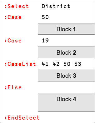
Fig. 5.17 A diagram with the usage of :Select, :Case and :CaseList.#

Remark

Values specified in :Case or :CaseList clauses can be numbers, characters or even nested arrays.

Here is an example using all of those:

∇ arg ← CasePotpourri arg
    :Select arg
    :CaseList 'yes' 'no' 'doubt'  ⍝ 3 possible values
        ⎕← 'yes no doubt'
    :CaseList (2 7)(5 1)'Null'    ⍝ 3 different possible vectors
        ⎕← 'some vector'
    :Case 'BERLIN'                ⍝ 1 single word
        ⎕← 'Germany'
    :CaseList 'PARIS'             ⍝ 5 possible letters
        ⎕← 'A French letter'
    :Else
        ⎕← 'no match...'
    :EndSelect
∇

CasePotpourri 'yes'

yes no doubt yes

CasePotpourri 2 7

some vector 2 7

CasePotpourri 'I'

A French letter I

CasePotpourri 'BERLIN'

Germany BERLIN

CasePotpourri 'PARIS'

no match... PARIS

Be careful with the last three examples where a character vector is used, and the relevant :Case 'BERLIN' and :CaseList 'PARIS' clauses in the tradfn:

if the keyword is :Case, the control value must match the entire character vector “'BERLIN'”; and
if the keyword is :CaseList, the control value may be any one letter out of the five letters in “'PARIS'”. Any subset, like “'PAR'” will not be recognised as matching.

Warning

The control value must be strictly identical to the value(s) specified in the :Case clause(s), i.e. the result of using ≡ with the control value and the matching value in the clause should be 1.

For example, in the preceding diagram, there is a clause :Case 50 (scalar). If the control value is equal to 1⍴50 (a one-item vector), it is not strictly identical to the specified array (the scalar 50) and the corresponding set of statements will not be executed. In fact,

50≡(1⍴50)

0

5.7.4. Predefined Loops#

5.7.4.1. Basic Use (`:For`/`:In`/`:EndFor`)#

In many iterative calculations a set of statements is repeated over and over again, and on each iteration a new value is given to a particular variable. We will refer to this variable as the control variable.

If the values of the control variable can be predefined before the beginning of the loop, we recommend that you use the :For clause, with the following syntax: :For controlVariable :In listOfValues.

The keyword :For is followed by the name of the control variable. In the same statement, the keyword :In is followed by an expression returning the list of values to be assigned to the control variable on each iteration. Here is an example:

∇ r ← ZapMe y
    r ← 0
    :For zap :In 50 82 27 11
        ⎕← zap
        r ← zap
    :EndFor
∇

ZapMe 3

50 82 27 11 11

The block of statements between the :For and :EndFor will be executed 4 times: once with zap ← 50, then with zap ← 82, then with zap ← 27, and finally with zap ← 11.

Generally, the block of statements makes some reference to the control variable, for example as part of a calculation, but this is not mandatory.

This technique has one great advantage: the number of iterations is predefined, and it is impossible to accidentally program an endless loop.

5.7.4.2. Control of Iterations#

The values assigned to the control variable can be whatever values are needed by the algorithm:

a list of numeric values like 66+4×⍳20;
a nested vector like (5 4)(3 0 8)(4 7)(2 5 9);
a list of letters like 'DYALOG'; or
a list of words like 'Madrid' 'Paris' 'Tokyo' 'Ushuaia'.

It is also possible to use a set of control values, rather than just a single one.

For example, with :For (code qty) :In (5 8)(2 3)(7 4) the loop will be executed:

first with code ← 5 and qty ← 8;
then with code ← 2 and qty ← 3; and
finally with code ← 7 and qty ← 4.

In most cases, this kind of iterative process is executed to completion. However, it is possible to take an early exit when some condition or other is met. This can be done using the :Leave clause or using an explicit branch, like will be explained later.

A special variant of :In named :InEach is explained in Section 5.16.8 at the end of this chapter.

Example

Let us try to find all the possible divisors of a given integer.

A possible solution is to check the remainder of that value against all integers starting from 1, up to the number itself. If the remainder is 0, the integer can be appended to the vector of results, which has been initialised as an empty vector:

∇ divs ← Divisors n; rem; div
    divs ← ⍬
    :For div :In ⍳n
        rem ← div|n
        :If rem=0
            divs ← divs,div
        :EndIf
    :EndFor
∇

Divisors 3219

1 3 29 37 87 111 1073 3219

This example hopefully shows that it is straightforward to write simple, predefined loops using control structures. If you are used to other programming languages that do not offer array processing features, you may even find this way of writing programs very natural.

However, it turns out that many simple, predefined loops like this one are very tightly coupled to the structure or values of the data that they are working on: the number of items in a list, the number of rows in a matrix or, as in this example, the number of positive integers less than or equal to a particular value.

In such cases it is very often possible to express the entire algorithm in a very straightforward way, without any explicit loops. Usually the result is a much shorter program that is much easier to read and which runs considerably faster than the solution using explicit loops.

For example, in the example above it is possible to replace the loop by a vector of possible divisors produced by the index generator. The algorithm is unchanged, but the program is shorter:

]dinput
DivisorsNoLoops ← {
    (0=(⍳⍵)|⍵)/⍳⍵
}

DivisorsNoLoops 3219

1 3 29 37 87 111 1073 3219

and about 100 times faster:

]runtime -c 'Divisors 3219' 'DivisorsNoLoops 3219'

Divisors 3219 → 1.7E¯3 | 0% ⎕⎕⎕⎕⎕⎕⎕⎕⎕⎕⎕⎕⎕⎕⎕⎕⎕⎕⎕⎕⎕⎕⎕⎕⎕⎕⎕⎕⎕⎕⎕⎕⎕⎕⎕⎕⎕⎕⎕⎕ DivisorsNoLoops 3219 → 2.1E¯5 | -99%

The ]runtime -c is a user command that can be used to compare two or more pieces of code. It uses the first expression as the baseline and then compares the run time of the subsequent pieces of code against the first one. Here, the -99% on the second line means DivisorsNoLoops is 100 times faster, which can also be understood by comparing the run times (in seconds) of each expression, the 1.1E¯3 and 1.1E¯5 above (the exact numbers might fluctuate, depending on factors like how the CPU is feeling, the machine the code gets ran on, etc.)

Of course, sometimes the processing that is to take place inside the loop is so complex that it is infeasible to rewrite the program so that it doesn’t use an explicit loop. For example, the existence of a dependency such that the calculations taking place in one iteration are dependent on the results produced in the previous iteration will generally make it harder to write a program without an explicit loop.

5.7.5. Conditional Loops#

In the previous section we used the term “predefined loop” because the number of iterations was controlled by an expression executed before the loop starts. It is also possible to program loops which are repeated until a given condition is satisfied.

Two methods are available:

using :Repeat... :Until; and
using :While... :EndWhile.

The two methods are similar, but there are some important differences:

:Repeat:
- when the loop is initialised, the condition is not yet satisfied (generally);
- the program loops until this condition becomes satisfied;
- the “Loop or Stop” test is placed at the bottom of the loop; and
- the instructions in the loop are executed at least once.
:While:
- when the loop is initialised, the condition is (generally) satisfied;
- the program loops as long as it remains satisfied;
- the “Loop or Stop” test is placed at the beginning of the loop; and
- the instructions in the loop may not be executed at all.

5.7.5.1. Bottom-Controlled Loop (`:Repeat`/`:Until`)#

The control variables involved in the test are often initialised before the loop begins, but they can be created during the execution of the loop because the test is placed at the bottom.

Then the block of statements delimited by :Repeat... :Until is executed repeatedly up to the point where the condition specified after :Until becomes satisfied.

This condition may involve one or more variables. It is obvious that the statements contained in the loop must modify some of those control variables, or import them from an external source, so that the condition is satisfied after a limited number of iterations. This is the programmer’s responsibility.

Here is an example usage of :Repeat... :Until to calculate after how many years an investment reaches a target value, if it grows at a fixed rate:

∇ years ← rate ComputeGrowthTime values; amount; target
    years ← 0
    (amount target) ← values
    :Repeat
        amount ← amount×1+rate   ⍝ accumulate interest
        years ← years+1
    :Until amount≥target
∇

0.02 ComputeGrowthTime 10000 25000

47

0.03 ComputeGrowthTime 10000 25000

31

This means that if you invested 10.000 in an investment that grew 2% every year, then your investment’s value would surpass 25.000 after 47 years. If the growth rate is 3% instead, you would need 31 years instead.

The test is made on the bottom line of the loop, immediately after :Until, so the loop is executed at least once.

The “Loop or Stop” control is made at the bottom of each loop, but it is also possible to add one or more intermediate conditions which cause an exit from the loop using a :Leave clause or a branch arrow (this will be explained in Section 5.7.9).

special case

It is possible to replace :Until with :EndRepeat. However, because there is no longer a loop control expression, the program would loop endlessly. For this reason it is necessary to employ intermediate tests to exit the loop when using this technique.

5.7.5.2. Top-Controlled Loop (`:While`/`:EndWhile`)#

Because the test is now placed at the top of the loop, control variables involved in the test must be initialised before the loop begins.

Then the block of statements limited by :While/:EndWhile will be executed repeatedly as long as the condition specified after :While remains satisfied.

This condition may involve one or more variables. It is obvious that the statements contained in the loop must modify some of those control variables so that the condition is satisfied after a limited number of iterations. This is the programmer’s responsibility.

As an example, let us implement a function that takes a positive integer and computes its “Collatz path”. The Collatz path of a positive integer is built by starting at the number given and then:

if the number \(n\) you are at is odd, go to \(3n + 1\); or
if the number \(n\) you are at is even, go to \(\frac{n}{2}\).

The Collatz conjecture states that any positive integer eventually goes to 1. This tradfn can help us visualise this:

∇ path ← CollatzPath n
    path ← 1⍴n
    :While path[≢path]≠1
        n ← path[≢path]
        n ← ((n÷2) (1+3×n))[1+2|n]
        path ← path,n
    :EndWhile
∇

CollatzPath 1

1

CollatzPath 2

2 1

CollatzPath 11

11 34 17 52 26 13 40 20 10 5 16 8 4 2 1

The test is made in the top line of the loop, immediately after :While, so it is possible that the block of statements inside the loop will never be executed. In our case, when CollatzPath is called with 1 as its argument.

The “Loop or Stop” control is made at each beginning of a new iteration but it is also possible to add a second control at the bottom of the loop, replacing :EndWhile with a :Until clause, just like we did for the :Repeat loop.

5.7.6. Exception Control#

5.7.6.2. Leave the Loop (`:Leave`)#

This clause causes the program to stop the current iteration and to skip any future iterations, aborting the loop immediately, and continuing execution from the line immediately below the bottom end of the loop.

:Leave works with any kind of loop.

5.7.6.3. Jump to Another Statement (`:GoTo`)#

This clause is used to explicitly jump from the current statement to another one, with the following syntax: :GoTo destination.

In most cases, destination is the label of another statement in the same program.

A label is a word placed at the beginning of a statement followed by a colon. It is used as a reference to the statement. It can be followed by an APL expression, but for readability it is recommended that you put a label on a line of its own. For example, in

Next:
val ← goal-val÷2

Next is a label. Next is considered by the interpreter to be a variable whose value is the number of the line on which it is placed. It is used as a destination point both by the traditional branch arrow and by the :GoTo clause, like this: :GoTo Next is equivalent to →Next (cf. Section 5.7.8). Be careful not to include the colon after the branch name when referencing to it after a :GoTo or after a →.

5.7.6.3.1. Jump Destinations#

The following conventions apply to the destination of a jump:

`destination`	Behaviour of executing `:GoTo destination` or `→destination`
Valid label	Skip to the statement referenced by that label.
`0`	Quit the current function and return to the calling environment.
`⍬`	Do not jump anywhere but continue on to the next statement.

5.7.6.4. Quit This Function (`:Return`)#

This clause causes the tradfn to terminate immediately and has exactly the same effect as →0 or :GoTo 0. Control returns to the calling environment.

5.7.7. Endless Loops#

Whatever your skills you may inadvertently create a function which runs endlessly. Usually this is due to an inappropriate loop definition.

However, sometimes APL may appear to be unnecessarily executing the same set of statements again and again in an endless loop, when in fact it just has to process a very large amount of data or perform some heavy calculations.

Fortunately you can interrupt the execution of a function using two kinds of interrupts: weak and strong. Let us see what this means.

5.7.7.1. A Slow Function#

Let us consider the function below:

∇ Endless; i
    i ← 0
    :Repeat
        ⎕DL 3
        ⊢i ← i+1
    :Until i=20
∇

This function is not really endless, but the line ⎕DL 3 makes it DeLay all execution for (approximately) 3 seconds, so the whole loop should take about a minute to finish execution. (You will learn more about ⎕DL and related functions later down the road.)

The line ⊢i ← i+1 has the final ⊢ so the iteration number is printed as the loop progresses. However, if you are running the Jupyter Notebook version of this chapter, the numbers only show up after the iterations are all complete. This is due to a current shortcoming of the Dyalog APL kernel.

Don’t run this function yet!

5.7.7.2. Weak and Strong Interrupts#

If you issue a weak interrupt, the computer will complete the execution of the statement that it is currently processing. Then it will halt the function before executing the next statement. We recommend using a weak interrupt whenever possible because it allows the user to restart the function at the point it was interrupted (cf. the chapter with the first aid kit).

If you issue a strong interrupt, the computer will complete the execution of the APL primitive that it is currently processing. Then it will interrupt the function before executing the next primitive.

For example, in the Endless function above, it could calculate i+1 and stop before executing the assignment i ← i+1. Of course, if the user restarts the statement, it will be executed again in its entirety (it is impossible to resume execution in the middle of a statement).

Note that it is impossible to interrupt the execution of a primitive like i+1 itself, and sometimes the execution of some primitives may take a long time.

5.7.7.3. How Can You Generate an Interrupt#

If you are using the Windows IDE, by going to “Action” ⇨ “Interrupt” you can issue a weak interrupt. Similarly, RIDE’s “Action” ⇨ “Weak Interrupt” will do the trick.

In order to issue a strong interrupt, you either:

go to “Action” ⇨ “Strong Interrupt” if you are using RIDE; or
if you are using the Windows IDE, go to the system tray, look for the Dyalog APL icon, click it and then select “Strong Interrupt” (cf. Fig. 5.18).

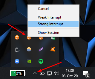
Fig. 5.18 Issuing a strong interrupt in the Windows IDE.#

The method explained above for the strong interrupts on the Windows IDE also works for weak interrupts. Be patient! If Dyalog APL is doing some heavy calculations for you, there may be a few seconds delay from when you click the APL icon until the menu shown above appears.

After you issue an interrupt (weak or strong) there may be a few more seconds delay before the interrupt actually occurs.

Now, let’s test it.

5.7.7.4. First a Weak Interrupt#

Start running the function and, after a couple of iterations, issue a weak interrupt as you learned in the previous section.

Sadly, the Jupyter Notebook interface has limited capability for dealing with interrupts, so for the remainder of this explanation you will be presented with some figures to illustrate the process.

If we define the tradfn on the Windows IDE, run it and then hit “Action” ⇨ “Interrupt”, what happens is illustrated in Fig. 5.19.

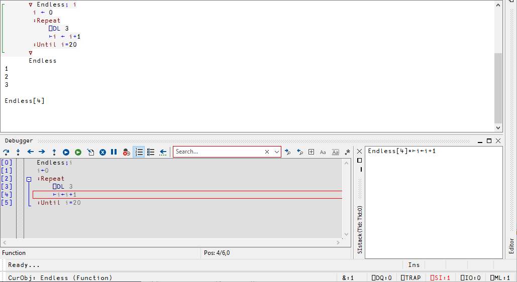
Fig. 5.19 A weak interrupt issued in the Windows IDE.#

Notice the Endless[4] message is below the few iteration numbers that were printed, and the stack trace window (that opened at the bottom) has highlighted that same line: line 4. This means that the function has been interrupted just before executing line number 4, and you can be sure that line 3 has finished.

To back out from the interrupted state of execution, press the Esc key as many times as needed, or execute the command )reset, which will be explained shortly.

5.7.7.5. And Now a Strong Interrupt#

Run the function again, and after some time issue a strong interrupt.

The result should be slightly different, as you can see in Fig. 5.20:

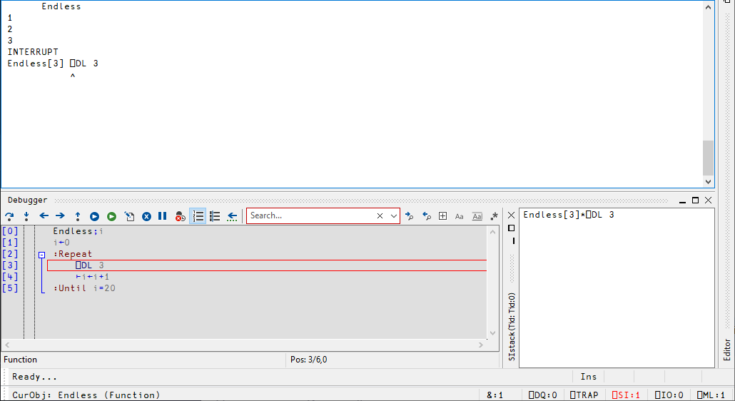
_images/Win_Endless_Strong_Interrupt.png

Fig. 5.20 A strong interrupt issued in the Windows IDE.#

This time, the message Endless[3] ⎕DL 3 tells you the line it was executing when it got interrupted, and the caret sign tells you which operation was being carried over. In this case, we did not let the 3 second delay finish.

5.7.8. Traditional Flow Control#

In early versions of APL, a unique symbol - the branch arrow (→, typed with APL+]) - provided the only means to override the order in which statements were executed. Today you should only use this mechanism when maintaining code which is already written in this style.

The branch arrow works in exactly the same way as the :GoTo clause. →destination and :GoTo destination are strictly equivalent.

destination should always be a label. Remember: a label is a word placed at the beginning of a statement and followed by a colon. Specifying a statement number (i.e. →47) would become incorrect as soon as you add or remove lines before that line number.

5.7.8.1. Equivalence With Modern Flow Control#

Using small tricks makes it possible to use → to emulate the modern keywords that control the flow of a program. Figuring out how to emulate all the keywords can be an interesting educational exercise but those tricks should be avoided in modern code.

As an example, we will see how we can emulate an :If... :EndIf clause. For that, you need to remember that jumping to an empty destination does nothing (cf. Section 5.7.6.3.1), so that statements are executed sequentially.

Consider the following program:

∇ money ← price IsItExpensive money
    →(~price≤money)⍴expensive  ⍝[1]
    money ← money-price        ⍝[2]
    expensive:                 ⍝[3]
∇

13 IsItExpensive 20

7

13 IsItExpensive 10

10

The program above uses (~price≤money)⍴expensive to emulate an :If clause and the expensive: line acts as the :EndIf clause. If you have enough money to buy something that costs price, it will return how much money you have left after making the purchase. If you don’t have enough money, your money is returned unchanged.

Let us walk through the execution of the two example calls above to see exactly how this works:

13 IsItExpensive 20:
- expensive is the label that is defined on line 3, so its value is 3 as if it were a regular variable;
- price≤money is 1 because 13≤20 and hence ~price≤money is 0;
- (~price≤money)⍴expensive is thus equivalent to 0⍴3 which evaluates to ⍬; and
- →⍬ does nothing (as explained in Section 5.7.6.3.1) and the program proceeds to lines 2 and 3.
13 IsItExpensive 10:
- expensive is the label that is defined on line 3, so its value is 3 as if it were a regular variable;
- price≤money is 0 because 13≤10 is not satisfied, hence ~price≤money is 1;
- (~price≤money)⍴expensive is thus equivalent to 1⍴3 which evaluates to 3; and
- →3 makes the program jump to line 3, skipping line 2.

This kind of conditional jump can be summarised like →(~condition)⍴ destination.

Using control structures, we would have written

∇ money ← price SaneIsItExpensive money
    :If price≤money
        ⎕← 'I have enough money'
        money ← money-price
    :EndIf
∇

13 SaneIsItExpensive 20

I have enough money 7

13 SaneIsItExpensive 10

10

or even better, without control structures at all we could write

]dinput
IsItExpensiveDfn ← {
    ⍵-⍺×⍺≤⍵
}

13 IsItExpensiveDfn 20

7

13 IsItExpensiveDfn 10

10

This example above shows that programming without explicit control flow is something that is quite feasible and, often times, very elegant.

In your road to mastering Dyalog APL you will want to train your brain to write programs more like the IsItExpensiveDfn above and less like the SaneIsItExpensive, and definitely not like the labelled IsItExpensive!

5.7.8.2. Multiple Destinations#

One can also use → with multiple labels on the right, in which case program execution jumps to the first label in the vector of labels. Just consider the following dummy program, where we use explicit line numbers so we can print them as the tradfn executes:

∇ MultipleDestinations
    →4 3 2 7
    2
    3
    4
    5
    6
    7
    8
∇

MultipleDestinations

4 5 6 7 8

Try changing the numbers in front of the → above and see how the numbers printed change.

5.7.9. Modern and Traditional Controls Cooperate#

It is sometimes convenient to mix modern and traditional flow control in order to simplify the code.

Consider a loop in which we must terminate the execution of the function if the condition x<3 becomes satisfied. With modern control structures, the function would probably include a

...
:If x<3
    :Return
:EndIf
...

which takes up 3 lines. This might be a bit cumbersome. It is possible to use fewer statements using an explicit branch:

...
:GoTo (x<3)/0
...

or equivalently

...
→(x<3)/0
...

since the branch arrow and the :GoTo keyword are equivalent.

Something very similar could be written if we need to leave a loop when a given condition becomes satisfied. For example, instead of

:Repeat
    ...
    :If cond
        :Leave
    :EndIf
    ...
:EndRepeat
...

one could write

:Repeat
    ...
    →cond/hell
    ...
:EndRepeat
hell:
...

Remark

Branching using → or :GoTo is not recommended as a general tool for programming flow control. It is briefly explained here mainly in order to help you understand existing code and to show that the technique may be useful and feasible in special situations. You should, in general, either use control structures or avoid them altogether with alternative formulations of your algorithm(s).

Warning

Colons are placed before a keyword (e.g. :For) but after a label (e.g. hell: above).

5.8. Dfns Versus Tradfns#

5.8.1. Comparison#

Having seen how dfns and tradfns work in practice, it is time to compare their main characteristics, so that we can understand what are the use cases in which each of them shines.

Characteristic	dfns	tradfns
Argument names	`⍺` is the left argument and `⍵` is the right argument.	The names are specified in the header of the function.
Reassigning the arguments	Disallowed, except to define default left argument.	Allowed.
Return value	The value of the first statement whose value is not assigned to a variable.	The value of the variable specified in the header.
Shy result	Last expression needs to be an assignment and must be followed by the closing `}`.	Enclose the header variable in `{}`.
Variable scope	Local by default.	Global by default.
Traditional flow control	Limited to usage of guards, in the form of `condition: statement`.	Complex flow control with control structures such as `:If`, `:For`, and `:While`.
Scoping	Lexical.	Dynamic.

5.8.2. Use Cases#

Based on the characteristics of both dfns and tradfns, there a few rules of thumb that help determine the situations in which dfns are more suitable and the situations in which tradfns are more suitable. Please, bear in mind that these are just guidelines to help you pick the right tool for the job, but ultimately the choice is yours and will boil down to your experience, personal preference, the context you are programming in, etc.

As already mentioned before, dfns shine when one wants to create a user-defined function with a clean and well-defined data flow, taking some arguments in and processing them to produce a result. Functions of this sort are usually such that they always return the same value when given the same arguments, which means you can have a high degree of confidence that the function works as expected provided you test it thoroughly.

Tradfns are very helpful when you need to create a more complex function, or something that resembles a script in other languages, and you simply need the type of flow control that tradfns offer. In those cases, it makes sense to have a tradfn that represents the program you want to create, and then the tradfn itself calls several other functions (that could very well be dfns) that process the arguments and do useful things with them. On top of that, if you have a complex function that is not working as it should, you may find it easier to debug if it contains control structures rather than if the flow control of the program were controlled by recursion or operators: with control structures you get more fine-grained control over where in the code you want to start debugging and how to do it. We will explore these ideas in more detail in the “First Aid Kit” chapter.

From the characteristics of both types of user-defined functions, it also follows that if you want to create a relatively short function, a dfn is probably the best option: dfns are very simple to define and the definitions themselves take up little space (as opposed to tradfns whose headers take up more space, especially if you then localise all the variables you use – which you generally should). As an example, in Dyalog’s annual APL problem solving competition, the first ten problems usually have a one-line solution, and those have to be submitted as dfns.

5.9. Input, Output and Format#

Up to now, our functions processed values passed as arguments, and returned results which could be used in an expression, assigned to a variable, or displayed. But a function can also get data from other sources and/or it can produce results which are not APL variables, but, for example, printed material or data files. In this section you will learn some useful techniques to write such functions.

This section will also help you use data that you may have already have stored in Excel worksheets or in text files on disk.

5.9.1. Some Input and Output Methods#

Here are some of the most typical methods used by a function to get input data or output results.

Some Input/Output methods	Input	Output	cf.
Display a result returned at function completion		X
Display intermediate values during execution		X	Section 5.9.3
Use or modify a global variable	X	X	Section 5.9.4
Exchange data with a spreadsheet (e.g. Microsoft Excel)	X	X	Section 5.9.5.3
Read or write data from/to a file (or a database)	X	X	Section 5.9.6
Print data on a printer		X	Section 5.9.7
Exchange data with a graphical user interface	X	X	Section 5.9.8
Get data typed by the user on the keyboard	X		Section 5.9.9
Use Internet facilities to get/send data	X	X	Section 5.9.10

Not all of these possibilities will be explained here; we shall limit our investigations to some simple methods that you may test immediately, using some utility functions we define for you. “I/O” is a common abbreviation for “input and output”.

We also provide some text files and spreadsheets that you can use for experimentation:

a CSV file BasicCarSales.csv;
text files mlk.txt and report.txt.

We recommend that you place those files in a reference directory where they will be preserved, and copy them to a test directory where you will be able to make some experiments and modify them at will. You can get these helper files from here.

We also suggest that you create a global variable in your WS with the path to that test directory, to avoid repeating it in all the tests you will do.

For example, we will set

filepath ← 'C:/Users/rodri/Documents/Dyalog/MDAPL/../res/testfiles/'

We recommend that you set this global variable with the absolute path to the folder as it is easier to get an absolute path to work.

In the following sections we will refer to this variable filepath.

5.9.2. Format#

In the preceding pages we found that we can display, on the screen, any kind of results: numbers, text or a mixture of numbers and characters in nested arrays. Now we shall try to output data to external media, like graphic interfaces, disk files or printers. Most of those media only accept text. For example, it is impossible to send numbers to a printer: we must first convert them to printable characters.

The APL language includes two such conversion tools: a function named format, represented by the symbol ⍕ and typed with APL+’, and a system function named ⎕FMT. You can remember ⍕’s position on the keyboard because ⍕ transforms its argument into a character array, and you input characters with a quote ', hence ⍕ is APL+’.

These facilities will be studied in detail in a subsequent chapter but we will introduce here the basic use of format.

5.9.2.1. Monadic Format#

Monadic format converts any array (numbers, characters and nested arrays) into its character representation. The result is exactly the same as what you see when you display the array in the APL session, because in fact, APL internally uses monadic format to display arrays:

character values are not converted: they remain unchanged; and
numeric and nested values are transformed into vectors or matrices of characters.

Here are some examples:

⍴⍕'album'

5

⊢chemistry ← 3 5⍴'H2SO4CaCO3Fe2O3'

H2SO4 CaCO3 Fe2O3

⍴chemistry

3 5

⍴⍕chemistry

3 5

'album' and chemistry are left unchanged because they are character arrays.

However, the 3-item numeric vector

⍴52 69 76

3

becomes an 8-item character vector once converted:

⍴⍕52 69 76

8

In a previous chapter we used a 2 by 3 nested matrix named nesMat:

⊢nesMat ← 2 3⍴'Dyalog' 44 'Hello' 27 (2 2 ⍴ 8 6 2 4) (2 3⍴1 2 0 0 0 5)

┌──────┬───┬─────┐ │Dyalog│44 │Hello│ ├──────┼───┼─────┤ │27 │8 6│1 2 0│ │ │2 4│0 0 5│ └──────┴───┴─────┘

Notice this matrix has 2 rows and 3 columns:

⍴nesMat

2 3

Once converted into text, it will become 20 characters wide and it will span 3 rows, because the second row of nesMat contained two small matrices:

⍴u ← ⍕nesMat

3 20

Dyalog 44 Hello 27 8 6 1 2 0 2 4 0 0 5

5.9.2.2. Dyadic Format#

Dyadic format applies only to numeric values. It converts them into text in a format controlled by the left argument, which is made up of two numbers:

the first number indicates the number of characters (the width of the output) to be used to represent each numeric value; and
the second number indicates how many decimal digits will be displayed.

Let us make some experiments with the following matrix:

⎕RL ← 73
⊢nm ← (?3 4⍴200000)÷100

21.21 1534.88 375.46 704.5 1125.14 1963.52 464.45 1438.25 796.53 1569 157.14 886.59

For example, if we want each number to be right aligned in a field with 8 characters of width and with 2 decimal digits, we’d use

8 2⍕nm

21.21 1534.88 375.46 704.50 1125.14 1963.52 464.45 1438.25 796.53 1569.00 157.14 886.59

The result has of course 3 rows and 32 columns (4 times 8 characters):

⍴8 2⍕nm

3 32

Instead, we may prefer to have each number in a cell 6 characters wide, with no decimal digits:

6 0⍕nm

21 1535 375 705 1125 1964 464 1438 797 1569 157 887

⍴6 0⍕nm

3 24

Remark

Values are not truncated, but rounded.

As an example, consider the second value of the first row:

nm[1;2]

1534.88

5 0⍕nm[1;2]

1535

Remark

Any attempt to apply dyadic ⍕ to characters will cause a DOMAIN ERROR.

Format will be studied in detail in a later chapter.

5.9.3. Displaying Intermediate Results#

During normal execution, most applications do not use the session window (the development environment); all input/output is typically done with more user-friendly interfaces. However, during the development of an application, it may be useful for experimental or debugging purposes to have a function display intermediate results.

This can be accomplished in 2 different ways:

inside a tradfn, if the result of an expression is not assigned to a variable it gets displayed;
- in particular, if you add ⊢ to the beginning of any line, that line will display its value, even if the line is an assignment (e.g. the line ⊢v ← 2×3 will assign 6 to v and display it);
any intermediate result can be displayed by assigning it to the quad symbol (⎕, typed with APL+l), and this assignment can even be placed in the middle of statements to check intermediate values:

v ← (⎕←chemistry[1;],chemistry[3;]),⎕←,chemistry[⎕←⍸chemistry='2']

┌───┬───┐ │1 2│3 3│ └───┴───┘ 22 H2SO4Fe2O3

Because we used ⎕← three times, three values got displayed one after the other, on three successive lines of the screen, in the order that they were evaluated:

First ⍸chemistry='2',
then ,chemistry[⍸chemistry='2']
and then chemistry[1;],chemistry[3;].

We recommend that you use this last method, which is the most explicit and which can be easily detected by any text search utility function. Following a similar reasoning, the use of implicit output by adding ⊢ to the left end of a statement is discouraged:

⊢ cannot be used to print intermediate results;
⊢ cannot be used in dfns because a dfn will return if an expression has a ⊢ on the left end; and
uses of ⊢ for the purpose of implicit output cannot be easily searched for, because ⊢ might be used for other purposes.

5.9.4. Using Global Variables#

A function can use (as input) or modify (as output) the contents of one or more variables which are global to it. The variables may be completely global, or they may be local to a calling function (so-called semi-global variables).

For example, as we suggested earlier, a global variable may contain a path used by dozens of functions in a workspace:

filepath

C:/Users/rodri/Documents/Dyalog/MDAPL/../res/testfiles/

It will be possible for any function to use this path to prefix some file names, for example as

⎕← file1 ← filepath,'sales.xls'

C:/Users/rodri/Documents/Dyalog/MDAPL/../res/testfiles/sales.xls

⎕← file2 ← filepath,'customers.txt'

C:/Users/rodri/Documents/Dyalog/MDAPL/../res/testfiles/customers.txt

Storing common parameters, like a folder path, in global variables can often be very convenient. For example, it makes it very easy to have the system use another set of files without changing any functions. This technique can for example be used to switch between running on test data and on production data.

Similarly, a function can output values into global variables, which may be used by many other functions sharing the same workspace.

You must be very cautious when using this technique:

maintenance of functions using global variables is complex because it is difficult to keep track of the different statements which use or update those variables;
if an error occurs, and if several functions can modify these global variables, it may be very difficult to determine which of them had last modified a variable involved in the error; and
if function execution is interrupted and restarted, global values set before the interruption may conflict with new ones calculated in a different context. For example, if the function increments a global variable in line [1] but crashes in line [2], and you restart the function, you will have the global variable incremented twice instead of once, as you had expected. Such errors are very nasty, as they can lead to other errors or breakdowns much later in the execution. It can be close to impossible to find the causes of such errors in a systematic way.

Such a technique should be restricted to a limited number of variables, clearly identified and documented by any convenient method: a common name prefix, an automated system of references, etc.

Sometimes when starting an application it is necessary to read a lot of settings from a file and make the settings available to all the programs that constitute the application. In such a situation it would make sense to write a program to read the settings from the file and store them in global variables in the workspace.

Tip

Whenever possible, favour explicit exchange of values through arguments and results.

5.9.4.1. Global Constants#

Because of the reasons explained above, programmers are discouraged from writing new values to global variables, but from the text above it is also clear that global variables can be very useful.

In particular, it is often very useful to use global variables to store important pieces of information that are constant throughout the whole execution of your application. This way, these important pieces of information can be accessed from within your functions with ease. It is a common convention (and a convention that is not specific to APL) to name these global constants in all uppercase letters and to not update their values after the variable is initialised.

As an example, the folder in which our files reside can be declared as a global constant:

FILEPATH ← 'C:/Users/rodri/Documents/Dyalog/MDAPL/../res/testfiles/'

Notice that from the language point of view, FILEPATH is just like any other variable and it can be modified:

FILEPATH ← 2

So it is indeed up to the programmer to respect the convention or not. We will respect the convention and hence we’ll redefine FILEPATH to its original value:

FILEPATH ← 'C:/Users/rodri/Documents/Dyalog/MDAPL/../res/testfiles/'

5.9.5. Exchanging Data With a CSV File#

As per the Wikipedia,

A Comma-Separated Values (CSV) file is a delimited text file that uses a comma to separate values. Each line of the file is a data record. Each record consists of one or more fields, separated by commas. The use of the comma as a field separator is the source of the name for this file format. A CSV file typically stores tabular data (numbers and text) in plain text, in which case each line will have the same number of fields.

Even though the CSV format is not fully standardised, it is a fairly common format and is suitable for sharing simple data.

APL has many system functions for I/O with files, including a system function ⎕CSV to read and write data to CSV files.

5.9.5.1. Importing Data#

Reading data from a CSV file can be as simple as giving it the path to the file you want:

⎕← contents ← ⎕CSV FILEPATH,'BasicCarSales.csv'

FILE NAME ERROR: C:/Users/rodri/Documents/Dyalog/MDAPL/../res/testfiles/BasicCarSales.csv: Unable to open file ("The syste
m cannot find the path specified.")
      ⎕←contents←⎕CSV FILEPATH,'BasicCarSales.csv'
                 ∧

The return value is a matrix with one row per line of text in the file and one column per data entry:

⍴contents

VALUE ERROR: Undefined name: contents
      ⍴contents
       ∧

You can use ⎕CSV to read data and have it separate the header for you and convert columns into the appropriate data types. For example, we can tell ⎕CSV to convert columns 2, 3 and 4 to numbers and to split the header:

⎕← contents ← ⎕CSV (FILEPATH,'BasicCarSales.csv') '' (1 2 2 2) 1

FILE NAME ERROR: C:/Users/rodri/Documents/Dyalog/MDAPL/../res/testfiles/BasicCarSales.csv: Unable to open file ("The syste
m cannot find the path specified.")
      ⎕←contents←⎕CSV(FILEPATH,'BasicCarSales.csv')''(1 2 2 2)1
                 ∧

More advanced use cases of ⎕CSV can be found in the appropriate section or in the documentation page for ⎕CSV. As an exercise, open the docs for ⎕CSV (by clicking the link or typing ⎕CSV in your interpreter and then pressing F1) and try to understand what the 1 in (1 2 2 2) does. Learning to read documentation pages may seem daunting at first, but it is an acquired skill that is very helpful for programmers.

5.9.5.2. Exporting Data#

Exporting data to a CSV file is done in a similar fashion, by passing in the data as the left argument to ⎕CSV. The data given can be the whole table or a 2-element vector like above, where the first element is the data and the second one is the header. If the file didn’t exist already, one could write

contents ⎕CSV FILEPATH,'BasicCarSales.csv'

VALUE ERROR: Undefined name: contents
      contents ⎕CSV FILEPATH,'BasicCarSales.csv'
      ∧

to save contents in the specified file.

Because the file already exists, you can see that APL issues a FILE NAME ERROR. You can think of this as being similar to that prompt you get whenever you try to close a window with unsaved changes: it is annoying whenever you really want to close without saving and it asks you if you are sure, but you are glad it exists when you accidentally try to close the window amidst your work. To force ⎕CSV to overwrite an already existing file, you will first need to learn about variant in the “Operators” chapter.

5.9.5.3. Exchanging Data With an Excel Worksheet#

Many applications are based on an intelligent partnership between Excel and APL:

some users enter data in a set of worksheets with a predefined structure;
APL reads the sheets and processes the data with much greater power, precision and flexibility than Excel is capable of; and
finally, APL outputs results into one or more worksheets, in which the user can modify the presentation, define additional simple calculations and produce simple graphs.

However, this only works out of the box if your operating system is Windows. The “loaddata.dws” workspace, distributed as part of the Dyalog APL system, contains a set of professional grade functions to read from and write to text files, Excel workbooks, CSV files, SQL databases and XML files.

5.9.6. Reading or Writing a Text File#

Files can have many different formats. Some contain integer or decimal numbers, some contain APL variables (vectors, arrays, nested values) as we shall see in a future chapter, but most files contain plain text.

In this chapter, we shall limit our investigations:

to text files which can be viewed and modified using a basic text editor like Microsoft Notepad; and
to rather small files that can be read or written as a whole in a single operation (depending on your workspace size, you can easily read/write thousands of lines of text).

Such a file can be considered as a long vector containing special line separation characters (“carriage return” and/or “line feed”). For that reason, when edited with Notepad, they look more or less like APL character matrices.

Except for special purposes, to exchange data between APL and a text file, one needs to:

convert the read data from a file as a character vector into a more convenient APL character array (to read); or
convert an APL character array into a special character vector with embedded line separators (to write).

Those conventions require some techniques we haven’t seen yet. This is the reason why we give you some predefined functions. You will find them in a workspace named Files.dws delivered with Dyalog APL. It contains a namespace (you can read about namespaces in their chapter) which itself contains the functions. To use them, you must:

copy the namespace inside Files.dws into your active workspace (be careful with the case):

)copy files Files

C:\Program Files\Dyalog\Dyalog APL-64 18.2 Unicode\ws\files.dws saved Fri Mar 18 10:04:20 2022

and

set an access path to the namespace contents:

⎕PATH ← 'Files'

Here are 3 functions you might find useful:

ReadAllText reads the contents of a text file and returns a character vector. The lines of the text are separated by two special characters: carriage return and/or line feed. The syntax is result ← ReadAllText path,fileID:

⎕← dream ← ReadAllText FILEPATH,'mlk.txt'

FILE NAME ERROR: C:/Users/rodri/Documents/Dyalog/MDAPL/../res/testfiles/mlk.txt: Unable to open file ("The system cannot f
ind the path specified.")
ReadAllText[3] tn←name ⎕NTIE 0
                       ∧

ReadAllLines reads the contents of a text file and returns a nested vector of character vectors, one vector per line of text in the file. The syntax is result ← ReadAllLines path,fileID:

⎕← dreamLines ← ReadAllLines FILEPATH,'mlk.txt'

FILE NAME ERROR: C:/Users/rodri/Documents/Dyalog/MDAPL/../res/testfiles/mlk.txt: Unable to open file ("The system cannot f
ind the path specified.")
ReadAllText[3] tn←name ⎕NTIE 0
                       ∧

PutText writes a character matrix (or vector) to a file. If a file with the same name already exists, it is replaced by the new file. The function returns the number of characters written to the file. The syntax is number ← textMatrix PutText path,fileID:

⎕← number ← chemistry PutText FILEPATH,'chemistry.txt'

FILE NAME ERROR: C:/Users/rodri/Documents/Dyalog/MDAPL/../res/testfiles/chemistry.txt: Unable to open file ("The system ca
nnot find the path specified.")
PutText[14] tn←name ⎕NTIE 0
                    ∧

The workspace loaddata.dws, distributed as part of the Dyalog APL system, contains a set of professional grade functions to read from and write to text files, Excel workbooks, SQL databases and XML files. loaddata.dws contains two functions LoadText and SaveText to complement the set of functions described above. LoadText and SaveText are designed to work with comma separated files (.CSV files) and fixed field width text files.

We have only used text files. Dyalog APL also includes an advanced file system designed to work very easily and efficiently with APL arrays, as well as a generalised interface to SQL databases. The APL file system is described in its own chapter. The SQL interface is not described in this tutorial; please refer instead to the specialised brochures available here.

5.9.7. Printing Results on a Printer#

Printing your APL objects on paper should be avoided whenever possible, to help preserve the environment. If you really must print things to paper, there are a couple of alternatives you can consider.

Perhaps the simplest alternative is to generate a PDF with what you wish to print, and then print the PDF you generated.

If you are using the Windows Interpreter, you can easily print the contents of your workspace by going to “File” ⇨ “Print…”. From there, you can leave the defaults untouched and select a printer on the “Printer” tab. If you have a printer set up, you can choose it from the list of available printers. Otherwise, you can print to a PDF file. Please notice that the contents of the workspace that get printed are all of the named objects you have: variables, functions, operators, etc. If you just type 3 + 3 in the interpreter and execute it, that does not get printed with this method – to print the log you need to go to “Log” ⇨ “Print…”.

If you are not in the Windows interpreter or do not wish to print all of the contents of your workspace, you can use a different approach. For that, we have to use some functionalities of APL that you haven’t seen before. Explaining these in depth is outside the scope of this chapter, but we will give an overview of how it works.

Here is how I would print a character vector v to a PDF file to be saved in my Desktop, with the name 'test.pdf':

v ← 'This is just a character vector.'
path ← 'C:/users/rodri/Desktop/test.pdf'

r ← ⎕NEW 'HTMLRenderer' (('HTML' v)('Visible' 0))

r.PrintToPDF path

1

)erase r

What this is doing is creating a new (⎕NEW) object named HTMLRenderer that knows how to render, you guessed it, HTML. (HTML is the markup language in which websites are written.) We then give it the character vector and ask for the window to remain invisible, with ('Visible' 0). If we had written ('Visible' 1), a window like the one in the figure Fig. 5.21 would pop up:

Fig. 5.21 An HTMLRenderer object with a sentence.#

After the character vector is rendered, we print the contents of the window to the path specified and then we erase the temporary variable.

Printing an arbitrary array is slightly more involved, because we have to convert said arbitrary array to a suitable character vector first. Sadly, ⍕ may not do the job because ⍕ applied to high-rank arrays still yields high-rank arrays. In order to overcome this obstacle, we need to find a way of transforming arbitrary arrays into character vectors.

For this end, we will be using the format function ⍕ we learned about before and the system function ⎕UCS, that was used above in the exercise where you framed a character matrix. What we will do is use ⍕ to convert any array into a character matrix, then to the right of the matrix catenate the newline character (that we can produce with ⎕UCS 10) and then ravel everything so that we have a character vector instead of a character matrix. Finally, we wrap that character vector in a little bit of HTML code, so that the array displays nicely.

Process ← {matrix ← ⍕⍵ ⋄ vector ← ,matrix,⎕UCS 10 ⋄ '<pre>',vector,'</pre>'}

This Process dfn takes an array and creates a character vector that looks pretty much like the original, apart from the heading and trailing HTML code:

⎕← array ← 5 6⍴⍳30

1 2 3 4 5 6 7 8 9 10 11 12 13 14 15 16 17 18 19 20 21 22 23 24 25 26 27 28 29 30

⎕← v ← Process array

⍴v

101

Now we can print this character vector, representing our array, to a PDF:

r ← ⎕NEW 'HTMLRenderer' (('HTML' (Process array))('Visible' 0))

r.PrintToPDF path

1

)erase r

This creates a PDF file that looks like the one in Fig. 5.22. We can see array was properly formatted on the top left corner:

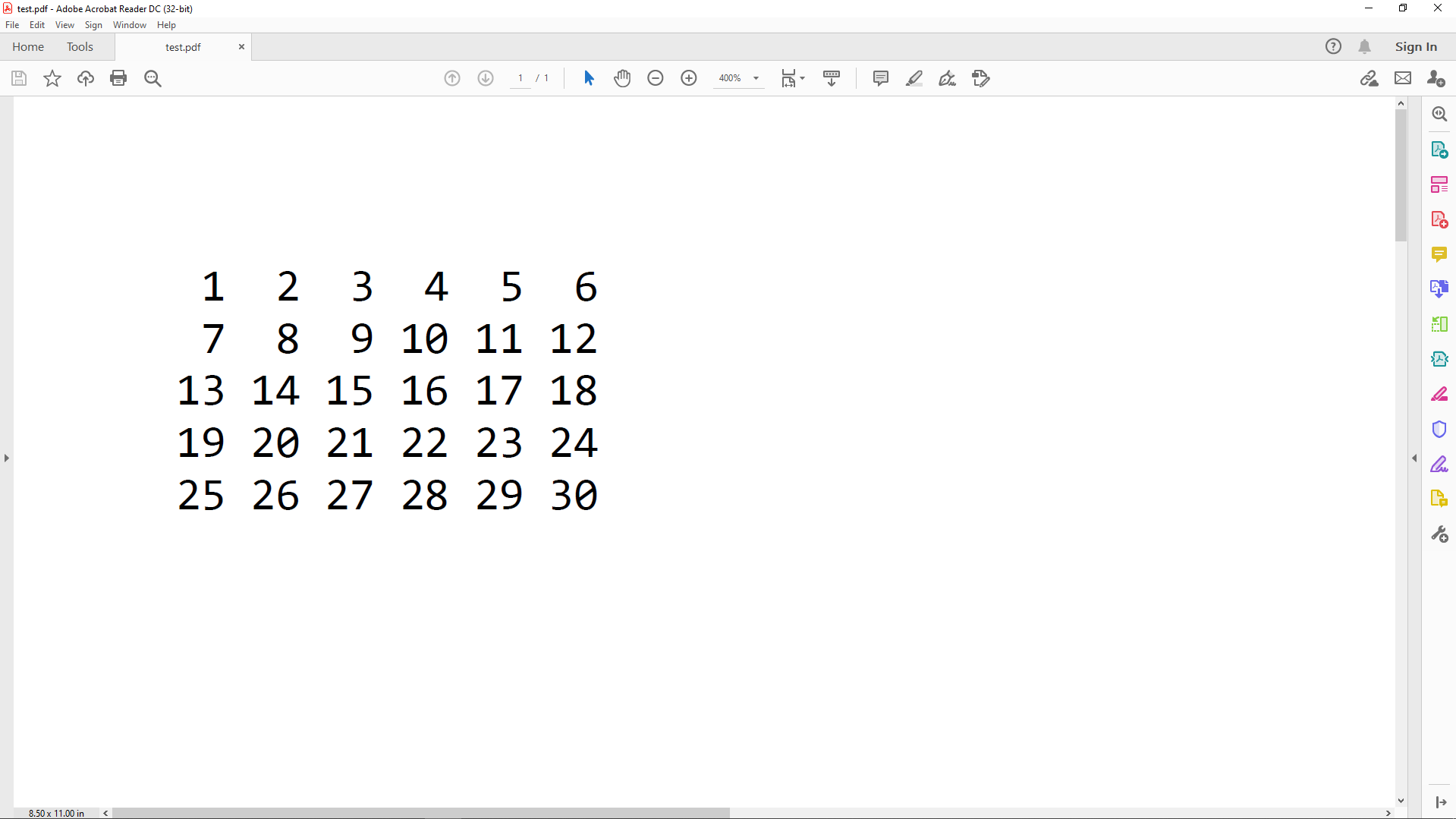
Fig. 5.22 array was printed to a PDF.#

Lastly, if you want to print a function Func, you can use the Process dfn on the vector representation ⎕VR of Func.

5.9.8. Using a Graphical User Interface#

We shall see in a later chapter how easy it can be to create graphical user interfaces (GUIs) which allow both input and output of information.

In the figure Fig. 5.23 we can see a basic GUI for a calculator. The user can press buttons to type in numbers (give input to the application) and to perform arithmetic operations on those numbers. After the results are calculated, they are shown in the white boxes at the top of the application (the application gives output to the user).

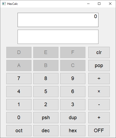
Fig. 5.23 A basic calculator written in APL.#

5.9.9. Requesting Values From the Keyboard#

Here again, if the user of an application is required to enter some input data, this is often done via some user-friendly GUI interface like the previous one or from a web page. However, during the development phase or for a light application it may be simpler to use a very basic question/answer mode.

Two symbols are used to request input from the user:

quad (⎕) is used to enter one or more numbers; and
quote-quad (⍞, typed with APL+Shift+[) is used to enter any string of characters.

5.9.9.1. Quad-Evaluated Input#

The first method is no longer in common use, but can be useful when prototyping an application which needs to request input. Also, you can easily accidentally type ⎕ in the session and activate quad-evaluated input, so it is worth studying it briefly.

Quad causes a pause in the execution of a function and allows the user to type any kind of expression. That expression is evaluated like any APL expression entered in the session, and its result is the result of the quad function:

when a function executes a quad, it displays ⎕: at the left margin of the screen to inform the user that he or she is expected to enter one or more values; and
if any error occurs during evaluation, the input quad is displayed over and over again, until the user succeeds in entering a valid expression.

In the following example, a function is supposed to count how many items of its right argument there are between two limits. These limits could be passed via a left argument, but in this case we choose to ask the user to enter them during execution of the function:

∇ Prompt1 vector; lim1; lim2; nb
    'What are the limits?'
    (lim1 lim2) ← ⎕
    nb ← +/(vector>lim1)∧(vector<lim2)
    (⍕nb),' values are comprised between ',(⍕lim1),' and ',⍕lim2
∇

As of the time of writing, Jupyter notebooks do not support input through ⎕ (nor through ⍞). We do encourage you to try these examples out for yourself somewhere other than the Jupyter Notebook interface.

    Prompt1 salaries
What are the limits?
⎕:
    1000 2000
4 values are comprised between 1000 and 2000

You can use this salaries variable:

⎕RL ← 73
⎕← salaries ← ?20⍴5000

2121 4778 4914 3139 4561 221 1252 1530 4475 332 3507 1829 1710 4964 3849 669 3653 3415 3867 151

Let us make an error while executing the function again:

      Prompt1 salaries
What are the limits?
⎕:
      mylims
VALUE ERROR: Undefined name: mylims
      mylims
      ∧
⎕:
      ⌊0.5+0.9 1.1×Average salaries    
0 values are comprised between 2472 and 3022

Notice that we tried to answer with a variable name but that variable does not exist. An error message is issued, which is not very user-friendly! Then the user is automatically requested again to provide a value.

Then we provide a valid value with an expression that makes use of a variable, a defined function and some primitives. The expression evaluates to 2472 3022 and those are the limits used.

Hint

If you accidentally start evaluated input in the session, type a → and then press enter, or type Space and then hit Enter to interrupt the input loop.

5.9.9.2. Quote-Quad Character Input#

Quote-quad allows the user to enter a string of characters. That string is returned as the result of the quote-quad function.

If the user types nothing and just presses the Enter key, the returned value is an empty text vector.

∇ Prompt2; tex
    'Type any string of characters'
    tex ← ⍞
    '"',tex,'" is a vector of length ',⍕≢tex
∇

     Prompt2
Type any string of characters
Are you serious?
"Are you serious?" is a vector of length 16

You can see that the quote-quad does not display any prompt sign.

Tip

Avoid using Quad evaluated input, as users can inadvertently (or intentionally) interfere with your own function variables.

Quote-Quad remains useful for quick tests, the development of light interactive functions or scripting applications which work with redirected I/O.

5.9.10. Fetching Data From the Web#

“Fetching Data From the Web” might mean several different things. It might mean to find, download and fix some APL code, it might be to download some data files or it might be to scrape websites for information. Different tools exist to cater to different needs.

The most basic way of fetching data from the web involves taking a URL and asking for the data that a browser would get if you typed that URL into the address bar.

As an example, consider Dyalog’s URL:

URL ← 'https://dyalog.com'

In order to fetch the data from that URL, we first need to load the HttpCommand namespace:

]load HttpCommand    ⍝ We use ] instead of ) here.

#.HttpCommand

Now we can simply type

data ← HttpCommand.Get URL

to fetch the data from the Internet. We can inspect the result:

data

[rc: 0 | msg: | HTTP Status: 200 "OK" | ⍴Data: 20667]

data is an object that contains all the information that we received when we requested the URL above. Usually, one is interested in the data.Data. For example, with a couple of lines of APL we can find links to all problem statements of the previous APL Problem Solving competitions:

URL ← 'https://www.dyalog.com/student-competition.htm'    ⍝ The URL where the problem sets are.
data ← HttpCommand.Get URL                                ⍝ Fetch the page.
base ← ⊃('<base +href="(.*?)"' ⎕S '\1') data.Data         ⍝ Find the base URL for the pdfs.
⎕← links ← ('href="(.*?[.]pdf)"' ⎕S (base,'\1')) data.Data  ⍝ Look for the pdf links and prepend the base.

┌─────────────────────────────────────────────────────────────────────────────────┬─────────────────────────────────────────────────────────────────────────────────┬─────────────────────────────────────────────────────────────────────────────────┬─────────────────────────────────────────────────────────────────────────────────┬─────────────────────────────────────────────────────────────────────────────────┬─────────────────────────────────────────────────────────────────────────────────┬─────────────────────────────────────────────────────────────────────────────────┬─────────────────────────────────────────────────────────────────────────────────┬─────────────────────────────────────────────────────────────────────────────────┬─────────────────────────────────────────────────────────────────────────────────┬─────────────────────────────────────────────────────────────────────────────────┬─────────────────────────────────────────────────────────────────────────────────┬─────────────────────────────────────────────────────────────────────────────────┬─────────────────────────────────────────────────────────────────────────────────┬─────────────────────────────────────────────────────────────────────────────────┬─────────────────────────────────────────────────────────────────────────────────┬─────────────────────────────────────────────────────────────────────────────────┬─────────────────────────────────────────────────────────────────────────────────┬──────────────────────────────────────────────────────────────────────────┬──────────────────────────────────────────────────────────────────────────┬──────────────────────────────────────────────────────────────────────────┬──────────────────────────────────────────────────────────────────────────┐ │https://www.dyalog.com/uploads/files/student_competition/2021_problems_phase1.pdf│https://www.dyalog.com/uploads/files/student_competition/2021_problems_phase2.pdf│https://www.dyalog.com/uploads/files/student_competition/2020_problems_phase1.pdf│https://www.dyalog.com/uploads/files/student_competition/2020_problems_phase2.pdf│https://www.dyalog.com/uploads/files/student_competition/2019_problems_phase1.pdf│https://www.dyalog.com/uploads/files/student_competition/2019_problems_phase2.pdf│https://www.dyalog.com/uploads/files/student_competition/2018_problems_phase1.pdf│https://www.dyalog.com/uploads/files/student_competition/2018_problems_phase2.pdf│https://www.dyalog.com/uploads/files/student_competition/2017_problems_phase1.pdf│https://www.dyalog.com/uploads/files/student_competition/2017_problems_phase2.pdf│https://www.dyalog.com/uploads/files/student_competition/2016_problems_phase1.pdf│https://www.dyalog.com/uploads/files/student_competition/2016_problems_phase2.pdf│https://www.dyalog.com/uploads/files/student_competition/2015_problems_phase1.pdf│https://www.dyalog.com/uploads/files/student_competition/2015_problems_phase2.pdf│https://www.dyalog.com/uploads/files/student_competition/2014_problems_phase1.pdf│https://www.dyalog.com/uploads/files/student_competition/2014_problems_phase2.pdf│https://www.dyalog.com/uploads/files/student_competition/2013_problems_phase1.pdf│https://www.dyalog.com/uploads/files/student_competition/2013_problems_phase2.pdf│https://www.dyalog.com/uploads/files/student_competition/2012_problems.pdf│https://www.dyalog.com/uploads/files/student_competition/2011_problems.pdf│https://www.dyalog.com/uploads/files/student_competition/2010_problems.pdf│https://www.dyalog.com/uploads/files/student_competition/2009_problems.pdf│ └─────────────────────────────────────────────────────────────────────────────────┴─────────────────────────────────────────────────────────────────────────────────┴─────────────────────────────────────────────────────────────────────────────────┴─────────────────────────────────────────────────────────────────────────────────┴─────────────────────────────────────────────────────────────────────────────────┴─────────────────────────────────────────────────────────────────────────────────┴─────────────────────────────────────────────────────────────────────────────────┴─────────────────────────────────────────────────────────────────────────────────┴─────────────────────────────────────────────────────────────────────────────────┴─────────────────────────────────────────────────────────────────────────────────┴─────────────────────────────────────────────────────────────────────────────────┴─────────────────────────────────────────────────────────────────────────────────┴─────────────────────────────────────────────────────────────────────────────────┴─────────────────────────────────────────────────────────────────────────────────┴─────────────────────────────────────────────────────────────────────────────────┴─────────────────────────────────────────────────────────────────────────────────┴─────────────────────────────────────────────────────────────────────────────────┴─────────────────────────────────────────────────────────────────────────────────┴──────────────────────────────────────────────────────────────────────────┴──────────────────────────────────────────────────────────────────────────┴──────────────────────────────────────────────────────────────────────────┴──────────────────────────────────────────────────────────────────────────┘

Don’t worry if you do not understand the APL code above (it is simpler than it might look, but explaining it is not the purpose of this section). You can see that the code returns some hyperlinks, which point to PDF files with the problem sets that we mentioned. You can read more about HttpCommand here.

5.10. Syntax Considerations#

5.10.1. Comments and Statement Separators#

5.10.1.1. Comments#

It is possible to write comments in a function to make it easier to read, explain how it should be used and help future maintenance or improvements.

Comments begin with the symbol lamp ⍝ (because it “illuminates” the code). Lamp can be typed with APL+,.

They can be placed alone on a dedicated line or to the right of any statement, including the function header. All the characters placed to the right of the lamp are ignored by the interpreter.

Tip

Determining when and where to comment your code is subjective but a good piece of advice is to try and not use comments to spell out what the code is doing; instead, consider using comments to explain why the code is doing what it is doing.

5.10.1.2. Statement Separators#

Several statements can be placed on the same line of a function, using the statement separator diamond ⋄, which can be typed with APL+`. Statements are executed starting from the leftmost one.

Putting several statements on the same line does not save computing time and generally does not improve the readability of a function. It should be reserved for short, straightforward statements.

The diamond separator can also be used in multithreaded programming to force the execution of a set of statements without any switch to another thread. But this is outside the scope of this tutorial.

As an example of the usage of comments and statement separators, consider a revision of the Interlace function we have seen above:

∇ r ← a Interlace b; size; even  ⍝ This is just a demo
    ⍝ a & b are matrices of the same shape
    size ← 1 2×⍴a     ⍝ the final result has twice as many columns as a
    r ← size⍴0
    even ← 2×⍳(⍴b)[2] ⍝ final indices of the columns of b
    r[;even] ← b ⋄ r[;even-1] ← a ⍝ interlace
∇

We have placed some comments: in the header, on a dedicated line and to the right of some statements. We have also grouped the last two statements on a single line, separated by a diamond.

5.10.2. Why Should a Function Return a Result?#

During the execution of a tradfn any result which is not assigned to a variable name is immediately displayed on the screen; we used that in our functions Prompt1 and Prompt2 above.

So, let us compare two very similar tradfns and their usage:

∇ z ← x Plus y
    z←x+y
∇

6 Plus 8

14

∇ x PlusNoRes y
    x+y
∇

6 Plus 8

14

Apparently, both functions work very well:

the left one calculates a local variable z, which has been declared to be the function result. The function returns the value of z as its result, and because the result is not assigned or used, it is displayed on the screen; and
the right one calculates x+y. Because this sum is not assigned, it is immediately displayed.

But now, let us try to include these functions in more complex expressions:

10×6 Plus 8

140

10×6 PlusNoRes 8

14
VALUE ERROR: No result was provided when the context expected one
      10×6 PlusNoRes 8
           ∧

Something went wrong!

the leftmost function returns a result. The result is available to the calling expression, in this case as the right argument to the multiply function, so that we obtained the answer we wanted; but
the rightmost function returns no result. The value calculated in the first statement is just displayed (though we did not need it); it is not returned as a result. So, the multiply function has an argument on its left (the 10) but nothing on its right, hence the error message.

Tip

Whenever you can, write functions which produce an explicit result. You can always throw the result away if you don’t need it.

This is not even a problem in dfns, because dfns always return an explicit result, or they don’t return at all. Because dfns are the more modern way of writing user-defined functions, and because we encourage you to write your functions that process data as dfns whenever possible, this is likely not to be a common problem for you.

5.10.3. Different Types of Functions#

5.10.3.1. What Is an Explicit Result?#

We have seen that some functions (like Average or Plus) return a result; we describe the result as being explicit. It means that once the function has been executed, the result is passed on to the next part of the expression which is being evaluated or, if there is none, it is displayed on the screen.

Some other functions (like PlusNoRes) do not return an explicit result. This does not mean that they do nothing; perhaps they read or write data from/to a file or an Excel worksheet, perhaps they print a graph on a printer, or perhaps they build a graphical user interface. All these consequences which arise from the execution of the function can be called implicit or hidden results. Anything that happens during the execution of a function and that is not communicated directly in the function’s result is generally called a side effect of the function (and perhaps its sub-functions).

5.10.3.2. Six Major Types of Functions (Valence)#

The number of arguments a function takes is termed its valence.

You have already met functions with one or two arguments (monadic or dyadic), and you can also write functions which take no arguments at all: they are called niladic. Though they do not receive values through arguments, they can process data introduced via the various techniques described in Section 5.9. Notice that only tradfns can be niladic, as dfns take at least one argument.

Depending on whether or not they return an explicit result, tradfns can be classified as follows:

Valence	With an explicit result	Without an explicit result
Niladic	`∇ z ← function`	`∇ function`
Monadic	`∇ z ← function x`	`∇ function y`
Dyadic	`∇ z ← x function y`	`∇ x function y`

Dfns, on the other hand, can only be of two different types: either monadic with an explicit result or dyadic with an explicit result.

Niladic functions which return no result are very similar to scripts written in other programming languages.

Some of the functions which we have already written can be classified as follows:

Syntax	With result	Without result
Niladic		`Endless`
Monadic	`Average`, `HarmonicMean`	`Prompt1`, `Prompt2`
Dyadic	`Interlace`, `Plus`, `Times`	`PlusNoRes`

5.10.3.3. Ambivalent Functions#

Most APL symbols are used to represent both monadic and dyadic primitive functions. For example, the symbol ⍴ represents both the shape (⍴y) function and the reshape (x⍴y) function, and ⌈ represents both ceiling (⌈y) and maximum (x⌈y). These symbols are said to be ambivalent.

In Section 5.3.4 we saw how to write an ambivalent dfn. To write an ambivalent tradfn, the name of the left argument in the header is specified within braces (to show that is is optional), like this: ∇ result ← {left} Function right.

We are now faced with a problem: this function must work correctly whether or not a left argument is provided. One of the ways to deal with this in a dfn is by specifying a default left argument. There is another way that works for both dfns and tradfns, and then there is an additional, preferred, way of dealing with this ambiguity in tradfns.

A way to test for the presence of the left argument is through the system function ⎕NC. NC stands for name classification, as that is what the ⎕NC function does: classifies the use that is being made of a given name.

As we shall see in a future chapter:

the name classification of a variable name is 2;
the name classification of a function name is 3;
the name classification of an unused name is 0.

As some examples, recall that 'chemistry' is the name of a variable, 'Average' is the name of a function and so far we haven’t used the name 'thingamabob' for anything:

⎕NC 'chemistry'

2

⎕NC 'Average'

3

⎕NC 'thingamabob'

0

So, we can use the expression 0=⎕NC'⍺' to check if a dfn was called monadically and, in the example above, use 0=⎕NC'left' to check if the tradfn was called monadically. Conversely, we can use 2=⎕NC'⍺' to check if a dfn was called dyadically and, in the example above, use 2=⎕NC'left' to check if the tradfn was called dyadically.

Just to check that it works, let us write a useless ambivalent dfn:

]dinput
Useless ← {
    0=⎕NC'⍺': 'monadic'
    2=⎕NC'⍺': 'dyadic'
    'uh, what..?'
}

23 Useless 78

dyadic

Useless 71

monadic

Can you see why this ⎕NC method is better suited for dfns than for tradfns?

In a dfn, the left argument is always called '⍺', whereas for a tradfn it can change. If you change the name of the left argument in the header of the function and forget to change its name in the ⎕NC test you can get into trouble. For that matter, it is recommended that you use a different method to check if a tradfn was called monadically: the 900 I-beam, or 900⌶ (where ⌶ is the I-beam character, typed with APL+Shift+1). The I-beam will be covered in more detail, here we ask you to close your eyes and just believe 900⌶ does what we tell you it does.

When used inside a tradfn, 900⌶⍬ returns 1 if the tradfn was called monadically and 0 otherwise.

5.10.3.4. Example Ambivalent Function#

The following tradfn rounds a numeric value to its nth decimal digit:

∇ r ← n Round val; t
    t ← 10*n
    r ← (⌊0.5+val×t)÷t
∇

2 Round 41.31875 82.92413 127.71625

41.32 82.92 127.72

2 0 3 Round 41.31875 82.92413 127.71625

41.32 83 127.716

Now, suppose that we usually want to round values to the second decimal digit: we can decide that if we do not specify a left argument this will be the default behaviour of our function. Here is the updated version of the function:

∇ r ← {n} Round val; t
    :If 900⌶⍬
        n ← 2    ⍝ default value if Round is called monadically
    :EndIf
    t ← 10*n
    r ← (⌊0.5+val×t)÷t
∇

Now the left argument is optional and an :If... :EndIf clause detects its presence. If absent, n is set to 2. The expressions shown below illustrate the two ways in which the function can be used. This function really is ambivalent.

2 0 3 Round 41.31875 82.92413 127.71625

41.32 83 127.716

Round 41.31875 82.92413 127.71625

41.32 82.92 127.72

Alternatively, consider writing a dfn in which providing a default left argument is much cleaner:

]dinput
Round ← {
    ⍺ ← 2
    t ← 10*⍺
    (⌊0.5+⍵×t)÷t
}

5.10.3.5. Shy Result in a Tradfn#

Like for dfns (cf. Section 5.5.2), tradfns can return a shy result: in the header of the function we enclose the name of the return variable with {}, like so:

∇ {r} ← x ShyFun y
    r ← x×y
∇

17 ShyFun 3

⎕← 17 ShyFun 3

51

10×17 ShyFun 3

510

5.10.3.6. An Argument Used as a Result#

It is possible to use the same name for the result as one of the arguments. For example, these are two valid headers: ∇ x ← x Fun y and ∇ y ← x Fun y.

This may be useful when a condition causes the function to terminate without any processing. Supposed that you want to repeatedly divide the right argument by 2, until the result becomes odd. A simple loop will do it, but if the argument is already odd, the loop stops immediately and the result is equal to the argument:

∇ y ← DivideIt y
    :While 0=2|y
        y ← y÷2
    :EndWhile
∇

If y is even the loop is executed at least once.

If y is odd the function exists immediately and returns the unmodified value of y as its result.

Of course this is only relevant for tradfns, as dfns do not return the value of a specific variable.

5.10.4. Nested Argument and Result#

5.10.4.1. Nested Right Argument#

Both the left and right arguments of a function can be nested vectors, as in Function 'London' 'UK' 7684700 40, for example.

A composite argument of this sort is often split (dispatched) into a number of separate local variables using multiple assignment, as illustrated in the following dfn:

]dinput
Dispatch ← {
    (town country population prefix) ← ⍵
    country
}

Dispatch 'London' 'UK' 7684700 40

UK

For tradfns, a more elegant way to achieve the same thing is to specify the composite nature of the argument directly, as follows:

∇ r ← Dispatch (town country population prefix)
    r ← country
∇

Dispatch 'London' 'UK' 7684700 40

UK

Using this syntax, the items of the right argument are automatically allocated into local variables, as you could see above.

Remark

This special syntax applies only to the right argument, not to the left one. If a nested vector is passed on the left it can be split (dispatched) by multiple assignment, as suggested earlier.

5.10.4.2. Choice of Syntax#

When a function Fun is to receive two values x and y, you now have the choice between two syntaxes:

dyadic x Fun y
monadic Fun (x y)

The dyadic way has the advantage that the function can be used with reduce, while the monadic version cannot.

For example, we can use Plus in this kind of expression:

Plus/14 10 52 1 12 43

132

5.10.4.3. Nested Result#

Similar notation can be applied to the result of the function. Suppose that you want to return a vector of 3 separate (local) variables (named one, two and three in the example) as the result of the function. One way is to declare that the function returns a single named result, and to assign the 3 local variables into the result before the function terminates. Another approach is to simply declare the structure of the result in the header as illustrated below. As these names (one, two and three) appear in the header, they are local.

We exemplify this in the next tradfn:

∇ (one two three) ← left NestedRes right
    one ← left+right
    two ← right[left]
    three ← two×one[1]
∇

3 NestedRes 12 45 78

┌────────┬──┬────┐ │15 48 81│78│1170│ └────────┴──┴────┘

It should be clear from the construct itself, but this special syntax also only applies to tradfns. In dfns, you would have to do something like:

]dinput
NestedRes ← {
    one ← ⍺+⍵
    two ← ⍵[⍺]
    three ← two×one[1]
    one two three
}

3 NestedRes 12 45 78

┌────────┬──┬────┐ │15 48 81│78│1170│ └────────┴──┴────┘

5.10.5. Choice of Names#

Function names (as well as argument and result names, if you are using tradfns) can be any valid APL name, for example ∇ cain ← adam PLUS eve or dumb ← man WITHOUT voice.

However, it is recommended that you use simple names, names that are easy to remember, and names that are consistent from one function to the other. This is especially important if several people have to maintain a common set of functions; any of them should be able to understand immediately which variables represent the arguments and which the result…

This recommendation is really about adopting a strict naming convention, and this applies to any serious programming project, whether it uses APL or not.

Here are some simple conventions that you might consider:

∇ z ← x Function y, often used by English-speaking developers;
∇ r ← g Function d, often used by French-speaking developers;
∇ r ← a Function b;
etc.

However, we advise you to adopt meaningful words to indicate the nature of the arguments, for example using numVec for numeric vectors or texMat for character matrices.

We also recommend that you avoid modifying the arguments in the body of the function, otherwise you could make maintenance much more difficult.

5.11. Recursion#

A function is recursive when it calls itself, generally to calculate a step of an algorithm from the results of its previous step.

For example, the factorial of \(n\) can be defined as \(n\) times the factorial of \(n-1\). Of course, some condition must specify when the process is supposed to stop. In our example, the factorial of 1 is not calculated, but set to 1. A recursive function could be written as follows:

]dinput
Fact ← {
    ⍵<2: 1
    ⍵×Fact ⍵-1
}

Fact 8

40320

Warning

Recursive solutions are generally very elegant, however:

because a function may call itself a great number of times before it reaches the exit condition, this technique may need a lot of memory if the function works on huge arrays;
when the function calls itself, the variables calculated during one step must not interfere with the calling context. You must carefully localise all your variables if you are using a tradfn – otherwise this is already done for you. Either way, this is the reason for possible large memory consumption, as the local variables in all recursions may exist at the same time.

A possible way to overcome some of these limitations is introduced in Section 5.16.9.

Beware that recursion is never mandatory. A recursive function can always be rewritten using looping or array-oriented techniques instead of recursion.

For example, one could write the dfn that follows:

]dinput
Fact2 ← {
    ×/⍳⍵
}

Fact2 8

40320

Notice that the dfn above is preferred over a tradfn with an explicit loop like a :For or a :While.

5.11.1. Recursion in Dfns#

Both dfns and tradfns can be recursive by calling themselves explicitly, like you saw above. However, if you are writing a dfn you can also use the special symbol ∇ (the del symbol) to represent this self-call.

Using this symbol in our Fact function, we’d write

]dinput
Fact ← {
    ⍵<2: 1
    ⍵×∇⍵-1
}

An implicit self-reference using ∇ needs less interpretative overhead and therefore it may execute more quickly. Moreover, it will continue to work even if the function is renamed.

5.12. Assigning Names to Functions#

You can give names to values, through the use of variables like

x ← 2

and you can define functions, like

TimesTwo ← {2×⍵}

but you can also associate a new name with an existing primitive, a user-defined function or a derived function. For example,

Rho ← ⍴
2 2 Rho 1 2 3 4

1 2 3 4

Times2 ← TimesTwo
Times2 10

20

Sum ← +/
Sum 1 2 3 4

10

Later on, in the chapter about Tacit Programming you will see that you can even assign more primitives to a name, and those will behave in a very specific way.

Remark

When assigning a new name to an existing tradfn, the contents of the original function are not duplicated.

For example, here is a basic tradfn:

∇ r ← Add3 y
    r ← y+3
∇

And now we assign it a new name:

NewName ← Add3

If we check NewName’s code, it will be Add3’s source code:

NewName

∇ r←Add3 y [1] r←y+3 ∇

And finally, if we modify Add3, NewName also gets modified:

∇ r ← Add3 y
    r ← y+30
∇

NewName 10

40

Tip

If you accidentally assign a function to a new name when you wanted to use that name for a value, you can use )erase to fix that.

For example, say you typed this in your interpreter and accidentally pressed Enter:

Val ← Average

But what you really wanted to type was:

Val ← Average 41 11 19

SYNTAX ERROR: Invalid modified assignment, or an attempt was made to change nameclass on assignment
      Val←Average 41 11 19
      ∧

You can see that gives a SYNTAX ERROR because you are trying to change Val from a function to a value, and the interpreter doesn’t want you to do that.

Instead, first erase Val with

)erase Val

and then assign it normally:

Val ← Average 41 11 19

5.13. About the Text Editor#

Most of the features of the built-in Dyalog APL editor are very familiar to those of other common editors, but some are very specific and we therefore provide a brief description of the specific editing facilities of Dyalog APL.

5.13.1. Invoking the Text Editor#

Double-clicking a name which represents an existing item invokes the editor and displays its contents, using the colour scheme appropriate for the type of the item (function, character matrix, nested array, etc) defined via “Options” ⇨ “Colors…” if you are using the Windows interpreter or via “Edit” ⇨ “Preferences” ⇨ “Colours” if you are using RIDE.

You can also invoke the editor by pressing Shift+Enter when the input cursor is inside or adjacent to the name. This is perhaps the most convenient way as, when working in an APL session, you tend to use the keyboard much more than the mouse.

Let us define a character matrix with the uppercase latin alphabet:

⎕← charMat ← 2 13⍴⎕A

ABCDEFGHIJKLM NOPQRSTUVWXYZ

For some items (e.g. numeric matrices, some nested arrays) the editor is only good for viewing them, while for others such as functions, text vectors and text matrices, the editor can also be used to edit them. In Fig. 5.24 we have invoked the editor, and changed the contents of our charMat variable:

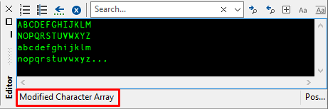
_images/Win_Editor_Edit_Character_Matrix.png

Fig. 5.24 Editing a character matrix with the built-in editor of the Windows interpreter.#

In Fig. 5.24 the edit window tells us that we modified the character matrix. We must now fix it, like we did with dfns before, for the variable to reflect its new value. RIDE doesn’t tell you that the character matrix was modified, but you still need to fix it if you want the new changes to come into effect.

If we now fix the changes to charMat, it will become a matrix with 4 rows and 29 columns (the length of its longest row).

If, for some reason, you made a mistake, you can exit the edit window without fixing the changes by pressing Shift+Esc.

If a name is currently undefined (has no value), double-clicking or pressing Shift+Enter on that name invokes the editor on it as if it were a new function. This is one way to create a function.

You can also invoke the editor using the command )ED as we did before. By default, it opens a function definition, but you can explicitly specify the type of a new object by prefixing its name with a special character, as shown in the table below.

Prefix	Example	Object Created
none	`)ed new`	Function
`∇`	`)ed ∇ borscht`	Function
`-`	`)ed - papyrus`	Simple character matrix
`→`	`)ed → crouton`	Simple character vector
`∊`	`)ed ∊ grunt`	Nested vector of character vectors, with one sub-vector per line

See also Section 14.2 for additional prefixes.

It is possible to open several edit windows using a single command. For example, )ed Tyrex -moose will open two edit windows. The first to create or edit a function named Tyrex and the second to create a character matrix named moose.

If a prefix is specified for the name of an already existing object, the prefix is ignored and the editor is invoked according to the type of the existing object.

There are some other ways to invoke the editor:

use ⎕ED instead of the command )ED. For example: ⎕ED 'Clown'. ⎕ED is a System function, a concept that will be discussed in a future chapter;
type a name, or put the input cursor on an existing name, and activate the menu “Action” ⇨ “Edit”;
for the Windows interpreter, type a name or put the input cursor on an existing name, and click the “Edit Object” available in the toolbar (cf. Fig. 5.25).

5.13.2. What Can You Edit?#

The following table shows the different item types that can be displayed using the text editor. Some of them can be modified (are “Editable”) while others cannot: they can only be viewed.

The table contains a list of the item types, the default foreground and background colours used to represent them and a “Yes” or “No” depending on whether they can be modified or not.

Item type	Foreground	Background	Editable
Function	various	White	Yes
Character matrix	Green	Black	Yes
Character vector	Black	White	Yes
Vector of character vectors	Blue	Black	Yes
Any numeric array	White	Grey	No
Mixed array	Blue	Grey	No
Object representation (`⎕OR`)	White	Red	No

5.13.3. What Can You Do?#

5.13.3.1. Cut / Copy / Paste#

it is possible to Cut / Copy / Paste text inside an edit window but also from one edit window to another one. It is also possible to copy text from the session window and paste it into any function, operator or editable variable, or vice-versa. So, if you have entered some experimental expressions in the session you can drag and drop them into a defined function.

On Windows, if you installed the default keyboard layout that comes with Dyalog APL, it may happen that Ctrl+c produces an APL glyph instead of copying the selected text. If this is the case, you can either install a layout that doesn’t have these collisions, like abrudz’s AltGr layout, or you can right-click and then select Cut / Copy / Paste, instead of using the usual keyboard shortcuts.

5.13.3.2. Drag/Drop Restrictions#

You may move or copy test using drag/drop but the following behaviour applies:

if you drag/drop within the same Edit window, the default operation is a move. If you press the Ctrl key at the same time, the operation is a copy;
if you drag/drop text from one window to another window, the operation is always a copy;
if you drag/drop text within the Session window, the operation is always a copy.

5.13.3.3. Exit the Editor#

We have already seen the main ways of leaving the editor:

press the Esc key (or use “File” ⇨ “Exit (and Fix)” on the Windows editor). This fixes the modifications and closes the edit window;
press Shift+Esc (or use “File ⇨ “Exit and discard changes” on the Windows editor). This leaves the editor without saving modifications; they are lost;
on Windows, “File” ⇨ “Fix” fixes the modifications but does not close the edit window.

5.13.4. Undo, Redo, Replay#

5.13.4.1. Undo#

As long as the contents of an Edit window have not been fixed, it is possible to undo all the modifications made since the last fix.

To undo modifications you can

press Ctrl+Shift+Backspace as many times as needed, or
activate the menu “Edit” ⇨ “Undo”.

If your APL keyboard layout allows it, you can also use Ctrl+z.

5.13.4.2. Redo#

Having used undo, it is possible to restore the changes that you have undone, one by one.

To redo modifications, you can

press Ctrl+Shift+Enter as many times as needed, or
activate the menu “Edit” ⇨ “Redo”.

If you APL keyboard layout allows it, you can also use Ctrl+y.

It must be emphasised that the Undo/Redo facility applies only to the current window. If some pieces of text have been copied to another window, the contents of the other window are not affected by the Undo or Redo operations.

5.13.4.3. Replay Input Lines#

The same keyboard shortcuts (Ctrl+Shift+Backspace and Ctrl+Shift+Enter) can be used to scroll up and down the statements that you have previously entered into the session window. For example, suppose you have made several sequential calculations that generate a considerable amount of output, only then to realise you made a mistake in the beginning.

You could scroll back through the considerable amount of output to find the statement with the error. However, you can search just through the input statements instead (only the lines that you have entered, excluding any output), which are stored in a dedicated Input History buffer:

press Ctrl+Shift+Backspace to scroll back through the Input History Buffer as many times as needed;
press Ctrl+Shift+Enter to scroll forward if you went too far back.

Once you have found the line, you can change it (or not) and then execute it again by pressing the Enter key.

If you are using the Windows interpreter, you can control the size of this dedicated buffer with the following configuration parameter: “Options” ⇨ “Configure…” ⇨ “Session” ⇨ “History buffer size”

5.14. Miscellaneous#

5.14.1. List of Variables and Functions#

You can obtain a list of your variables by typing

)vars

FILEPATH URL Val a actual array b base c charMat chemistry d file1 file2 filepath forecast hours inverses links mat nesMat nm path salaries times towns u v var which x zap

and you can obtain a list of your functions by typing

)fns

AMHM AbsVal Add3 Average BadSyntaxTradfn CasePotpourri CheckVar CollatzPath Comment ComputeGrowthTime ContinueInsideWhile Count Dispatch DivideIt Divisors DivisorsNoLoops Endless Fact Fact2 HarmonicMean Hypo Interlace IsItExpensive IsItExpensiveDfn Magic MultipleDestinations MultiplyBy10 NestedRes NewName Plus PlusNoRes PrintAB PrintCD PrintE Process Prompt1 Prompt2 QuadRoot Rho Root RootOf10 Round SaneIsItExpensive SetAThenPrint SetBThenPrint SetCThenPrint SetDThenPrint SetLocalE ShyFun Sign Silly Sum Times Times2 TimesTwo TradHarmonicMean Useless VarLevels ZapMe

5.14.2. Use of the Result#

To sum up what we have already seen, once a function has been defined and we call it, its result can be:

Immediately displayed and lost:

HarmonicMean times

0.895522

Included in an expression:

60×HarmonicMean times

53.7313

Assigned to a variable:

hours ← HarmonicMean times

5.14.3. Vector Representation#

We saw that double-clicking on a function name invokes the editor and allows the user to edit the code. We can also type the name of the function and see its code:

TradHarmonicMean

∇ mean←TradHarmonicMean argVector;inverses [1] inverses←÷argVector [2] mean←÷+/inverses ∇

One can also obtain this representation (as a character array) using the built-in system function ⎕VR (for vector representation) of Dyalog APL. System functions are a special kind of function provided with the development environment. The first character of their name is a quad (⎕) which guarantees that they cannot conflict with user-defined names, and their names are also case-insensitive:

⎕VR 'TradHarmonicMean'

∇ mean←TradHarmonicMean argVector;inverses [1] inverses←÷argVector [2] mean←÷+/inverses ∇

⎕Vr 'TradHarmonicMean'

∇ mean←TradHarmonicMean argVector;inverses [1] inverses←÷argVector [2] mean←÷+/inverses ∇

⎕vr 'TradHarmonicMean'

∇ mean←TradHarmonicMean argVector;inverses [1] inverses←÷argVector [2] mean←÷+/inverses ∇

⎕vR 'TradHarmonicMean'

∇ mean←TradHarmonicMean argVector;inverses [1] inverses←÷argVector [2] mean←÷+/inverses ∇

Note that this is quite unusual in a programming language. The result of ⎕VR is a character vector representing the source code of our function, which is now available for processing by other functions in the workspace!

System functions will be discussed in detail in a later chapter.

5.14.4. Source Code Management#

Up to now, all the functions and operators we defined were created with an APL code editor and stored in an APL workspace.

This monolithic one-workspace approach to application development works well for small applications developed by single programmers, but is often inappropriate for large applications developed by single programmers. Some groups have tacked this problem by storing code in ancillary workspaces or special files. Code is then copied dynamically into the main workspace when required, using techniques that will be explained later.

Had the same application been developed in a more traditional language, programs would be entered and modified using a text editor, stored in separate text files, and maintained independently from one another under the aegis of a source code management system that allows the team of programmers to coordinate their activities and keep track of changes.

This type of application development approach is also available in Dyalog APL, using source code management systems like SALT (for Simple APL Library Toolkit) and Link.

These systems make it possible to store sets of APL functions, operators and variables in text files that may be edited and managed using either the built-in APL code editor or industry standard tools This makes it easier to share code between projects and teams of developers.

To take full advantage of this new technique of developing applications, you should first learn about Namespaces and related topics, notations and commands. For this reason, these tools will be studied later in the chapter about source code management.

Fig. 5.26 Person drowning in APL glyphs is reassured by someone else telling him about the “First Aid Kit” chapter.#

5.15. Exercises on Tradfns#

Exercise 5.11

Write a function which displays the greatest value in a numeric matrix, along with its position (row and column) in the matrix.

actual

89 166 420 508 12 23 111 453 177 365 284 352 349 192 329 115 515 374 160 467 234 519 485 283

MaxPlace actual

The greatest value: 519 in row 4, column 4

Exercise 5.12

Conversions from Celsius to Fahrenheit degrees and back can be done using the following formulas:

F ← 32+9×C÷5 converts from Celsius to Fahrenheit;
C ← 5×(F-32)÷9 converts from Fahrenheit to Celsius.

Program a function Convert that makes the conversion C→F or F→C according to its right argument.

86 32 212 Convert 'F-C'

30 0 100

30 0 100 ≡ 86 32 212 Convert 'F-C'

1

7 15 25 Convert 'C-F'

44.6 59 77

44.6 59 77 ≡ 7 15 25 Convert 'C-F'

1

Exercise 5.13

Summing the items of a vector is so simple in APL (+/vec) that one cannot understand why this simple problem needs a loop in traditional languages! Just for fun, can you program such a loop in APL? Use control structures.

260 ≡ LoopSum 31 37 44 19 27 60 42

1

Exercise 5.14

In exercise 3 you were asked to reverse the order of a vector of items. Even if it is a strange idea, can you do the same operation using a loop, moving letter after letter?

ReverLoop 'The solution without loop was much better'

retteb hcum saw pool tuohtiw noitulos ehT

'retteb hcum saw pool tuohtiw noitulos ehT' ≡ ReverLoop 'The solution without loop was much better'

1

Exercise 5.15

In a given numeric matrix with \(n\) columns, we would like to insert subtotals after each group of \(g\) columns (where \(g\) is a divisor of \(n\)).

Try to write a function SubSum to do that, following these 3 steps:

reshape the matrix so that it fits in \(g\) columns only, with the necessary number of rows to contain all the values;
catenate, on the right, the totals of each row; and
reshape again that new matrix to obtain the final result.

In the examples below, the original matrix appears in black and the subtotals appear in grey:

actual

89 166 420 508 12 23 111 453 177 365 284 352 349 192 329 115 515 374 160 467 234 519 485 283

3 SubSum actual should give

\[\begin{split} \begin{matrix} 89 & 166 & 420 &\color{grey}{675} & 508 & 12 & 23 &\color{grey}{543} \\ 111 & 453 & 177 &\color{grey}{741} & 365 & 284 & 352 &\color{grey}{1001} \\ 349 & 192 & 329 &\color{grey}{870} & 115 & 515 & 374 &\color{grey}{1004} \\ 160 & 467 & 234 &\color{grey}{861} & 519 & 485 & 283 &\color{grey}{1287} \end{matrix} \end{split}\]

and 2 SubSum actual should give

\[\begin{split} \begin{matrix} 89 & 166 &\color{grey}{255} & 420 & 508 &\color{grey}{928} & 12 & 23 &\color{grey}{35} \\ 111 & 453 &\color{grey}{564} & 177 & 365 &\color{grey}{542} & 284 & 352 &\color{grey}{636} \\ 349 & 192 &\color{grey}{541} & 329 & 115 &\color{grey}{444} & 515 & 374 &\color{grey}{889} \\ 160 & 467 &\color{grey}{627} & 234 & 519 &\color{grey}{753} & 485 & 283 &\color{grey}{768} \end{matrix} \end{split}\]

r ←    89 166 420 675 508  12  23  543
r ← r,111 453 177 741 365 284 352 1001
r ← r,349 192 329 870 115 515 374 1004
r ← r,160 467 234 861 519 485 283 1287
(4 8⍴r) ≡ 3 SubSum actual

1

r ←    89 166 255 420 508 928  12  23  35
r ← r,111 453 564 177 365 542 284 352 636
r ← r,349 192 541 329 115 444 515 374 889
r ← r,160 467 627 234 519 753 485 283 768
(4 9⍴r) ≡ 2 SubSum actual

1

Exercise 5.16

This is a very classic problem: we want to partition a text vector each time a given separator is found and make a matrix from these pieces. Implement this functionality in a monadic function Separate.

Please bear in mind that is exercise is very manageable if you let yourself use a couple of control flow structures. However, solving this exercise with a dfn requires you to make an ingenious use of a primitive we have covered previously.

'/' Separate 'You/will/need a/loop/to solve/this/exercise'

You will need a loop to solve this

Exercise 5.17

Remember when we talked about the “Collatz Conjecture” earlier on? Don’t worry if you don’t. Now, you will implement a function that takes a positive integer n and creates a vector of numbers by successively taking the most recent number and then creating the next value according to a couple of rules:

if the most recent number is even, the next value will be half of it;
if the most recent number is odd, the next value will be 1 more than the triple of it; and
you stop when you reach 1.

CollatzPath 5

5 16 8 4 2 1

5 16 8 4 2 1 ≡ CollatzPath 5

1

CollatzPath 37

37 112 56 28 14 7 22 11 34 17 52 26 13 40 20 10 5 16 8 4 2 1

37 112 56 28 14 7 22 11 34 17 52 26 13 40 20 10 5 16 8 4 2 1 ≡ CollatzPath 37

1

5.15.1. Exercise Variants#

Now that you were given some exercises on dfns (cf. Section 5.4) and some exercises on tradfns (cf. Section 5.15), which ones can you solve with the other method? Solving exercises 11 to 17 with dfns will be harder than solving exercises 1 to 10 with tradfns.

Also, can you solve exercise 17 with a recursive function? Either dfn or tradfn, your choice.

5.16. The Specialist’s Section#

Each chapter is followed by a "Specialist's Section" like this one. This section is dedicated to skilled APLers who wish to improve their knowledge.

You will find here rare or complex usages of the concepts presented in this chapter, or discover extended explanations which need the knowledge of some symbols that will be seen much further in the book.

If you are exploring APL for the first time, skip this section and go to the next chapter.

5.16.1. Shadowed Names#

A name can be localised in a tradfn only if the programmer explicitly specifies its name in the function header. But a function can dynamically define new variables or new functions, using Execute (⍎) and ⎕FX.

So, during function execution, names of new variables and functions may be created dynamically. They could not therefore be localised explicitly when the function was written, but they can be localised, or shadowed, dynamically at runtime.

One or more names can be shadowed using the system function ⎕SHADOW, which accepts a vector of names separated by blanks, or a matrix of names with one name per row (but not a nested vector of names). For example, let us define a niladic tradfn Demonstration:

∇ Demonstration
    'This is just'
    'a demo function'
∇

and have dummy hold its canonical representation:

⎕← dummy ← ⎕CR 'Demonstration'

Demonstration 'This is just' 'a demo function'

Now that we have Demonstration’s canonical representation, we can erase the function from our workspace:

)erase Demonstration

Let’s now define a function Ombra with no localised names:

∇ vecRepr Ombra text
    ⎕SHADOW text,' ',vecRepr[1;]
    ⍎text,'←1'
    ⍎⎕FX vecRepr
    ⍝... ⍝ Intentional error.
∇

Let us execute it:

dummy Ombra 'new'

This is just a demo function

The function Ombra above

starts by shadowing the names new and Demonstration,
then dynamically creates a variable named new
and finally fixes a new function named Demonstration and executes it.

If you are using an interpreter, you can try uncommenting the final line of the Ombra tradfn so that the tracer interrupts function execution inside the tradfn. That way, you can check the names new and Demonstration have been created. But when the function completes, new and Demonstration disappear, as they were only local names:

new

VALUE ERROR: Undefined name: new
      new
      ∧

Demonstration

VALUE ERROR: Undefined name: Demonstration
      Demonstration
      ∧

5.16.2. Scoping in Nested Function Calls#

5.16.2.1. Reading the Caller’s Names#

We have seen that dfns have lexical scoping and that tradfns have dynamic scoping, but this can become complicated when we have dfns calling tradfns and tradfns calling dfns.

We will now try to answer the following question: when a function calls another independent function, can the callee read a name from the caller? We already know that if both the caller and callee are dfns, then the answer is no; on the other hand, if both the caller and the callee are tradfns, the answer is yes. In this exploration we will also show that the answer is yes for the cases when a dfn calls a tradfn and when a tradfn calls a dfn:

Can a callee ↓ read a name from the caller → ?	dfn	tradfn
dfn	No	Yes
tradfn	Yes	Yes

For our investigation we will define two “inner” functions (a dfn and a tradfn) that will act as the callee. Then we just need to write “outer” functions that act as the callers. To make our lives easier, all these functions will be dealing with a single variable named t, that we also set in the global scope:

t ← 'global var'

]dinput
InnerDfn ← {
    ⎕← t
    ⍬
}

InnerDfn⍬

global var

∇ x ← InnerTradfn x
    ⎕← t
∇

InnerTradfn⍬

global var

Now we create dfns and tradfns that assign locally to t, and then call the “inner” functions to see what value of t they actually print. We start by confirming the answers we already have, first by showing that if a dfn calls an independent dfn, then the callee cannot see the caller’s names:

]dinput
DfnCallsDfn ← {
    t ← 'DfnCallsDfn'
    InnerDfn⍬
}

DfnCallsDfn⍬

global var

Now we show that if the callee and the caller are tradfns, then the callee can read the caller’s names, even if the caller localises its names:

∇ x ← TradfnCallsTradfn x; t
    t ← 'TradfnCallsTradfn'
    InnerTradfn ⍬
∇

TradfnCallsTradfn⍬

TradfnCallsTradfn

Now we are left with the dfn-tradfn and tradfn-dfn cases:

]dinput
DfnCallsTradfn ← {
    t ← 'DfnCallsTradfn'
    InnerTradfn⍬
}

DfnCallsTradfn⍬

DfnCallsTradfn

∇ x ← TradfnCallsDfn x; t
    t ← 'TradfnCallsDfn'
    InnerDfn⍬
∇

TradfnCallsDfn⍬

TradfnCallsDfn

As we can see, with respect to accessing the caller’s variables, a dfn calling a tradfn and a tradfn calling a dfn behave in the same way as a tradfn that calls a tradfn, which confirms the table in the beginning of this sub-subsection.

It is worthwhile mentioning that the global value of t remains intact:

global var

5.16.2.2. Modifying the Caller’s Names#

It was shown before that a called function may read the value of the caller, but can it change its value? If the callee is a tradfn, you can change the value of the caller’s name with a plain assignment, because names in tradfns are not localised by default:

global var

∇ x ← InnerTradfn x
    ⎕← 'inner t: ',t
    t ← 'InnerTradfn'
    ⎕← 'inner t: ',t
∇

∇ x ← OuterTradfn x; t
    t ← 'OuterTradfn'
    ⎕← 'outer t: ',t
    _← InnerTradfn⍬
    ⎕← 'outer t: ',t
∇

OuterTradfn⍬

outer t: OuterTradfn inner t: OuterTradfn inner t: InnerTradfn outer t: InnerTradfn

]dinput
OuterDfn ← {
    t ← 'OuterDfn'
    ⎕← 'outer t: ',t
    _← InnerTradfn⍬
    ⎕← 'outer t: ',t
    ⍬
}

OuterDfn⍬

outer t: OuterDfn inner t: OuterDfn inner t: InnerTradfn outer t: InnerTradfn

However, if the callee is a dfn, plain assignment will create a new, local variable, with the same name as the one in the caller’s scope. That happens because names in dfns are local by default:

]dinput
InnerDfn ← {
    ⎕← 'inner t: ',t
    t ← 'InnerDfn'
    ⎕← 'inner t: ',t
    ⍬
}

∇ x ← OuterTradfn x; t
    t ← 'OuterTradfn'
    ⎕← 'outer t: ',t
    _← InnerDfn⍬
    ⎕← 'outer t: ',t
∇

OuterTradfn⍬

outer t: OuterTradfn inner t: OuterTradfn inner t: InnerDfn outer t: OuterTradfn

In this case, if you want to modify the name of the caller you have to trick APL into thinking you are reading from the name and writing to it at the same time, for example with a redundant modified assignment:

]dinput
InnerDfn ← {
    ⎕← 'inner t: ',t
    t ⊢← 'InnerDfn'    ⍝ Notice the modified assignment with ⊢
    ⎕← 'inner t: ',t
    ⍬
}

OuterTradfn⍬

outer t: OuterTradfn inner t: OuterTradfn inner t: InnerDfn outer t: InnerDfn

Once again, notice that the global t is still intact:

global var

These short explorations show that the scoping rules can become quite intricate, so it really is best to pass information in and out of functions as arguments/return values and not rely on scoping for that. This is, of course, just a suggestion and not a rule to follow blindly: a quintessential example of using scoping rules to your advantage is when defining a small inline dfn inside a larger function, e.g. to define a helper function that needs to be given as an operand to some operator, but that also needs access to the existing local variables.

5.16.3. Loop Control#

Loops programmed with traditional branch arrows are controlled by the APL statements. Loops using control structures are controlled by the interpreter. For that reason, if you trace loops programmed with :Repeat or :For, you will see that the first statement of the loop is executed only once, the following iterations execute only the “useful” statements. it is different for a :While loop because the test is placed in the first statement.

This has a surprising consequence. Imagine a :For loop using a control variable named again which is supposed to take three successive values: 12 54 86.

But the programmer erroneously alters the value of again during execution:

∇ Mess; again
    :For again :In 12 54 86
        again
        again ← 'Who modified me?'
        again
    :EndFor
∇

Mess

12 Who modified me? 54 Who modified me? 86 Who modified me?

Notice that, at each iteration, again is modified and is then automatically reset to the correct value in the subsequent iteration.

5.16.4. Labels and the Branch Arrow#

5.16.4.1. Niladic Arrow#

A niladic branch arrow → means: quit the current execution, i.e. quit the current function and all the calling functions, whatever the depth of the execution stack.

This is different from branching to zero →0 which means “quit the current function and resume execution in the calling environment”.

When an execution is interrupted, a niladic branch arrow clears its execution stack.

When an evaluated input is requested by a quad (⎕), a niladic branch arrow stops the request and forces an exit from the function and from all the calling functions.

Note, however, that a niladic branch arrow only clears the most current execution stack. If several functions have been interrupted and new ones started without first clearing the execution stack, you may have several active stacks. Each stack is identified by an asterisk to the right of the name of the interrupted function.

If you are running an interpreter, try defining the following functions:

]dinput
Foo ← {
    ... ⍝ Intentional error.
    ⎕
}

]dinput
Goo ← {
    Foo ⍬
}

If you run Goo⍬, you will get an error:

Goo⍬

SYNTAX ERROR
Foo[1] ... ⍝ Intentional error.
                               ∧

But if you are using an interpreter, the trace window should open and allow you to type APL expressions to debug your function. You can, for example, call Goo again, by typing Goo⍬ and then Goo⍬ again.

If, after that, you run )si, you get something like this:

      )si
#.Foo[1]*
#.Goo[0]
#.Foo[1]*
#.Goo[0]
#.Foo[1]*
#.Goo[0]

If you instruct the debugger to skip the current line (the line with ... that generates a SYNTAX ERROR) and to continue execution of the current thread, then APL will move on to the ⎕ line of Foo, in which you could do the following:

⎕:
      )si
⎕
#.Foo[2]
#.Goo[0]
#.Foo[1]*
#.Goo[0]
#.Foo[1]*
#.Goo[0]
⎕:
      →
      )si
#.Foo[1]*
#.Goo[0]
#.Foo[1]*
#.Goo[0]
      )reset
      )si

As you can see, several stacks were active and using → only cleared the most recent one. Using )reset cleared all the execution stacks in one go.

5.16.4.2. Branch to a Wrong Label#

We said that a label is processed as a numeric local variable which takes its value from the line number on which it appears. For example, if a function contains the statement next: newPrice ← oldPrice×(1-discount) on line [23], then next is a numeric value equal to 23. It is like a “read-only variable”, since you cannot modify it: any assignment to next would cause a SYNTAX ERROR. However, the value of next will change if some lines are deleted or inserted before line 23.

For this reason, the statements →next and :GoTo next are equivalent to →23 - but only as long as the label next is defined in line number 23!

We also said that a branch to zero causes an exit from the current function. This is also the case for any jump to a line number which is outside the number of lines in the function. For example, →50 would terminate any function which has less than 50 lines.

Now take a look at these two tradfns:

∇ MainFun
    SubFun
    ⎕← 'I''m back'
    ⍝ some empty line
    label: ⎕← 'Label line.'
∇

∇ SubFun
    :GoTo label
    ⎕← 'Can''t reach this'
∇

MainFun

I'm back Label line.

Here is what is going on:

When MainFun is executed, label immediately becomes a read-only variable whose value is 4.
When SubFun is called, label is local to MainFun but global to SubFun, so it is visible and is equal to 4.
When evaluated, the jump :GoTo label (or →next) is equivalent to :GoTo 4.
Because SubFun only has 2 lines, this jump terminates SubFun.
Execution then continues at MainFun[2], not at MainFun[4].

Conclusion: be very careful when using labels and non-localised names in general!

5.16.5. Other Conditional Execution#

In the course of this chapter, you have learned how to program conditional execution using control structures or traditional branching techniques.

APL provides two other methods: the function execute and the operator power.

5.16.5.1. Conditional Execution Using Execute#

The function execute (⍎) will be studied in more detail in a later chapter. It executes any character vector given as a right argument, as if it were an expression that had been typed into the APL session window. But if the vector is empty, nothing will be executed. This feature can be used to conditionally execute a statement. Let us consider the following expression:

diff ← 10 ⋄ limit ← 5
range ← ¯3 3
⍎(diff<limit)/'range ← ¯5 5'

range

¯3 3

diff ← 5 ⋄ limit ← 15
⍎(diff<limit)/'range ← ¯5 5'

range

¯5 5

If (diff<limit) is satisfied, 1/'range ← ¯5 5' gives 'range ← ¯5 5' and ⍎'range ← ¯5 5' will execute the expression, setting range to ¯5 5.

If (diff<limit) is not satisfied, then 0/'range ← ¯5 5' gives '' (an empty character vector) and ⍎'' does nothing, so range is not assigned.

Rule

More generally, one can write ⍎(condition)/text, where text is the quoted expression you want to evaluate conditionally.

When the expression on the right contains quotes, they must be doubled, and the expression may become more complex to read. Using execute will, in general, compromise the ability to analyse the code in order to, for example, search for references to a given function or global variable. For these reasons, and also because executed expressions run slightly slower than ordinary statements, this technique should be avoided. It is mentioned only because it has been used for years by many programmers, before better tools became available in APL.

Tip

Prefer control structures.

5.16.5.2. Conditional Execution Using the Power Operator#

The operator power (⍣, typed with APL+Shift+P) will be studied in more detail in a later chapter as well. It must not be confused with the function power (*).

Power can be used to execute a given function a set number of times. Of course, if we set that number to 1 then the function is executed once and if we set that number to 0, then the function is not executed at all. For example, in Section 5.10.3.4 we wrote a function which rounds a vector of values:

a ← 37
vec ← 17.4269 69.8731 82.3137
Round vec

17.43 69.87 82.31

(Round⍣(a>20))vec

17.43 69.87 82.31

In the expression above, (a>20) evaluates to 1 because a is 37, and hence Round is applied once.

If we change the test to something that evaluates to 0, then Round is not applied:

(Round⍣(a>80))vec

17.4269 69.8731 82.3137

We must separate the operator’s right operand from the resulting derived function’s argument.

We can use a “no-op” function like ⊢ as separator or use parentheses.

Rule

More generally, one can write {x} (Function⍣(condition)) y

5.16.6. Name Category#

The system function name category (⎕NC) indicates if a name currently represents a variable, a function, an operator and so on.

When applied to a nested vector of names, it returns an extended result, which gives more information. For example:

⎕NC 'Round' 'Foo'

3.2 3.2

3.1 means that Round is a tradfn;
3.2 means that Foo is a dfn;

Let us now assign some new names to some functions:

Round2 ← Round
Foo2 ← Foo
Rho ← ⍴
Sum ← +/

⎕NC 'Round2' 'Foo2' 'Rho' 'Sum'

3.2 3.2 3.3 3.3

This makes clear that:

assigning a new name to a user-defined function preserves its name category; and
primitive or derived functions have a name category equal to 3.3.

5.16.7. Bare Output#

When using quad (⎕) to input data, the prompt and the user’s answer appear on different lines on the screen.

When using a quote-quad (⍞) to input data, it is possible to force the system to issue the user with a prompt and collect their input on the same line of the screen. This is done by first assigning the prompt (a character vector) to ⍞ and then referencing ⍞. When the assignment and reference are performed like this, as successive operations, the system does not throw a newline after the prompt and the user input is collected on the same line as the prompt. This is called bare output.

Here is an example you can try in your interpreter: ⍞← 'This is my question: ' ⋄ z ← ⍞.

If you execute this and type something into the prompt, you will notice that z gets the complete line as value: prompt and user input.

Using take and drop, it is possible to remove the prompt, like in this demonstration function:

∇ info ← Demo; fn; na; cy
    ⍞← 20↑'First name ...................'
    fn ← 20↓⍞
    ⍞← 20↑'Name .........................'
    na ← 20↓⍞
    ⍞← 20↑'Country ......................'
    cy ← 20↓⍞
    info ← fn,' ',na,' ',cy
∇

And here is an example interaction (you can try it in your interpreter; Jupyter Notebook does not support ⎕/⍞ input at the time of writing):

      Demo
First name .........Charles
Name ...............Darwin
Country ............UK
Charles Darwin UK

We get all the prompts aligned and the return value only has the user’s inputs.

5.16.8. `:InEach`#

The control phrase :For... :In can be used to assign values to several control variables. One can also use :InEach which assigns one item from each of a set of nested values to the corresponding control variable. Sometimes :In is more convenient than :InEach and sometimes the reverse is true, as we will now show:

Let us assume that data for an invoice is represented as a number of lines, each with a quantity and a price:

invoice1 ← (10 100)(20 200)(30 300)

Then we process each line in a loop using this function:

∇ Process1 invoice
    :For (q p) :In invoice
        q×p    ⍝ "Process" this invoice line
    :EndFor
∇

Process1 invoice1

1000 4000 9000

Some day somebody decides to deliver the invoice data in a slightly different way: first all the quantities, then all the prices:

invoice2 ← (10 20 30)(100 200 300)

Then we only need to modify our processing function to use :InEach instead of :In:

∇ Process2 invoice
    :For (q p) :InEach invoice
        q×p    ⍝ "Process" this invoice line
    :EndFor
∇

Process2 invoice2

1000 4000 9000

Rule

In :For vars :InEach nesVec, ⍴vars is equal to the shape of nesVec, whereas in :For vars :In nesVec, ⍴vars is equal to the shape of each item in nesVec.

5.16.9. Tail Recursion#

As was outlined in Section 5.11, recursive solutions can be very elegant but may consume a lot of memory as successive calls accumulate local variables in their respective scopes.

For example, consider the following recursive definition of the factorial function:

]dinput
Factorial ← {
    ⎕← ≢⎕SI
    ⍵ ≤ 1: 1
    ⍵×∇⍵-1
}

Factorial 10

1 2 3 4 5 6 7 8 9 10 3628800

The Factorial function above makes use of ⎕SI, the state indicator, to tell how many functions are in the execution stack. Think of it as a pile of all the functions that are currently being executed, with the more recent calls at the top of the stack. As we can see, when we reach the deepest level of recursion (when ⍵ hits 1) we have 10 Factorial calls in the stack, which are then resolved as we return from deeper levels and perform the ⍵×... multiplication in the last line of the dfn.

A moment of reflection shows that, to compute the factorial of n with this function, the execution stack grows to size n. If our Factorial function were more complex, we would also have n copies of all the local variables the function would define. This duplication is what makes recursive functions potentially memory heavy. It is, however, something that the interpreter knows how to optimise in certain cases.

If we write a recursive function in such a way that the recursive call is the very last thing to be executed inside your function, then the interpreter knows it can discard everything from the current scope when it makes the recursive call. In fact, when we leave the recursive call we won’t have to do anything with the return value, as the recursive call was the very last thing we did in our function.

If we do this, then we are using a technique called tail recursion, because we are only recursing at the “tail” of the function.

Remark

Tail recursion is a feature of dfns and does not have an immediate equivalent in tradfns.

In the Factorial function above, the recursive call was in the last expression executed but it is not the last thing that is done in the function, as we have to multiply ⍵ with the return value of the recursive call. We can, however, refactor the function to carry temporary calculations in the left argument ⍺:

]dinput
TailFactorial ← {
    ⎕← ≢⎕SI
    ⍺ ← 1
    ⍵≤1: ⍺
    (⍺×⍵)∇⍵-1
}

TailFactorial 10

1 1 1 1 1 1 1 1 1 1 3628800

In this way, we can perform the multiplications as we go “down” the recursion, instead of waiting for the moment when we start coming back “up” again.

As an exercise, can you redo exercise 17 with a tail recursive function?

5.17. Solutions#

Solution to Exercise 5.1

If ⍵ is the vector argument, we can use ⍵[...] to index into ⍵ and then we can use the index generator primitive to generate the indices we need, which should be the integers from 1 to ⍺… Except that if ⍺ is too big, we cannot generate indices larger than the length of the vector, so we also find the minimum between ⍺ and ≢⍵. If we don’t, we get a INDEX ERROR when indexing. Here is a possible implementation:

]dinput
Extract ← {
    ⍵[⍳⍺⌊≢⍵]
}

3 Extract 45 86 31 20 75 62 18

45 86 31

6 Extract 'can you do it?'

can yo

20 Extract 1 2 3

1 2 3

Solution to Exercise 5.2

We can use a reasoning similar to that of the first exercise, except now we want to start the indices at ⍺+1 and go up until ≢⍵. For this to happen, we first need to find out how many numbers we need. If a vector has ≢⍵ elements and we are going to drop ⍺ of them, we are going to be left with (≢⍵)-⍺. This means ⍳(≢⍵)-⍺ will generate the correct amount of indices, but they will be starting at 1 and should start at ⍺+1, so we just need to add ⍺ to that.

Finally, we just need to worry about what happens if ⍺ is too large, i.e. if we want to ignore too many elements. The reverse of that concern is, what happens if (≢⍵)-⍺ is too small? Recall that (≢⍵)-⍺ tells you how many elements you will want to keep. But that number must be at least 0 elements (i.e. “keep no elements”) because it makes no sense to keep a negative number of elements. So we can just use ⌈ to find the maximum between 0 and (≢⍵)-⍺. If ⍺ is too large, 0⌈(≢⍵)-⍺ gives 0 and ⍳0 is the empty vector ⍬, so the indexing will work just fine.

]dinput
Ignore ← {
    ⍵[⍺+⍳0⌈(≢⍵)-⍺]
}

3 Ignore 45 86 31 20 75 62 18

20 75 62 18

6 Ignore 'can you do it?'

u do it?

20 Ignore 1 2 3

Solution to Exercise 5.3

This is another exercise on index arithmetic. Here is what we want to happen with a vector argument of length 10:

generate the indices 1 2 3 4 5 6 7 8 9 10
transform them into 10 9 8 7 6 5 4 3 2 1

We can do this if we do the correct subtraction:

11 - ⍳10

10 9 8 7 6 5 4 3 2 1

But here 11 was a special number: it was 1+≢⍵. So that is the general tactic we can employ:

]dinput
Reverse ← {
    ⍵[(1+≢⍵)-⍳≢⍵]
}

Reverse 'snoitalutargnoc'

congratulations

Reverse '!ti did uoY'

You did it!

Solution to Exercise 5.4

This exercise can be solved by using the operator reduce to sum: +/. Then we need to specify the axis we care about with [1] and [2].

If we do +/[1] then we are reducing across the first axis, which means we get the sums along the columns:

⎕← mat ← 3 4⍴75 14 86 20 31 16 40 51 22 64 31 28

75 14 86 20 31 16 40 51 22 64 31 28

+/[1]mat

128 94 157 99

We can then catenate the original matrix to these column sums vertically (by using ⍪), and then use +/[2] to find the row sums and catenate them with ,:

]dinput
Totalise ← {
    colSums ← +/[1]⍵
    r ← ⍵⍪colSums
    rowSums ← +/[2]r
    r,rowSums
}

Totalise mat

75 14 86 20 195 31 16 40 51 138 22 64 31 28 145 128 94 157 99 478

totMat ← 4 5⍴75 14 86 20 195 31 16 40 51 138 22 64 31 28 145 128 94 157 99 478
totMat ≡ Totalise mat

1

Solution to Exercise 5.5

When reading this exercise, one should immediately realise that we are going to need to find where the blank spaces are:

text ← 'This seems to be a good solution'

⍸' '=text

5 11 14 17 19 24

These indices tell where the blank spaces were in the character vector, and in between those indices are the indices that correspond to word characters:

the first word has indices 1 2 3 4
- then there is a space at position 5
the second word has indices 6 7 8 9 10
- then there is a space at position 11
…
- then there is a space at position 24
the last word has indices 25 26 27 28 29 30 31 32

The 32 above is ≢text:

≢text

32

From the list above we can see that most words are between spaces, but the first and last words may not be between spaces. We can fix this by forcing the first and last words to be between spaces if we add a single ' ' to the beginning and to the end of our variable:

⍸' '=' ',text,' '

1 6 12 15 18 20 25 34

Now we have

the first space at position 1
- the first word in positions 2 3 4 5
a space at position 6
- a word in positions 7 8 9 10 11
…
a space at position 25
- the last word in positions 26 27 28 29 30 31 32 33
the final space at position 34

So we can find the lengths of those runs of non-spaces by subtracting positions of consecutive spaces and then subtracting 1 from those, because 6-1 gives 5, but between 1 and 6 there’s only 4 integers.

]dinput
Lengths ← {
    spaces ← ⍸' '=' ',⍵,' '
    idx ← ⍳(≢spaces)-1
    ¯1+spaces[1+idx]-spaces[idx]
}

Lengths 'This seems to be a good solution'

4 5 2 2 1 4 8

The final step where we index into spaces to get “all but the last” and “all but the first” elements of spaces could have been done with your previous solutions:

]dinput
Lengths ← {
    spaces ← ⍸' '=' ',⍵,' '
    ¯1+(1 Ignore spaces)-((¯1+≢spaces) Extract spaces)
}

Lengths 'This seems to be a good solution'

4 5 2 2 1 4 8

Notice that doing ¯1+expr is a little “trick” you can employ when you want to subtract 1 from expr, but expr would then need parenthesis if you were to have it on the left of the - sign. For example, to subtract 1 from ≢spaces you would have to do (≢spaces)-1 but instead you can do ¯1+≢spaces.

Finally, can you improve your solution to handle multiple consecutive spaces?

Lengths 'This only    has      five words   '

4 4 0 0 0 3 0 0 0 0 0 4 5 0 0 0

Probably seeing how your function works with multiple consecutive spaces gives the solution away: consecutive spaces will make a 0 appear in the final result, so we just have to remove those:

]dinput
Lengths ← {
    spaces ← ⍸' '=' ',⍵,' '
    r ← ¯1+(1 Ignore spaces)-((¯1+≢spaces) Extract spaces)
    (0≠r)/r
}

Lengths 'This only    has      five words   '

4 4 3 4 5

Solution to Exercise 5.6

We have seen in Section 4.15.1 how to create any arithmetic sequence of integers. This is just a special case of the algorithm given, with Step ← 1:

]dinput
To ← {
    ⍺+¯1+⍳(1+⍵-⍺)
}

17 To 29

17 18 19 20 21 22 23 24 25 26 27 28 29

Solution to Exercise 5.7

This exercise is easier than it might look because the primitives to catenate vertically and horizontally, ⍪ and ,, know how to deal with a matrix and a single scalar:

⎕← towns ← 6 10⍴'Canberra  Paris     WashingtonMoscow    Martigues Mexico    '

Canberra Paris Washington Moscow Martigues Mexico

towns,'|'

towns⍪'-'

Canberra Paris Washington Moscow Martigues Mexico ----------

So we just have to frame the four sides and then change the corners:

]dinput
Frame ← {
    f ← '|',⍵,'|'
    f ← '-'⍪f⍪'-'
    (r c) ← ⍴f
    f[1 r;1 c] ← '+'
    f
}

Frame towns

Here we used the very convenient indexing notation f[1 r;1 c] that allows us to access the positions 1 1, 1 c, r 1 and r c of the matrix f.

Modifying this function to use the appropriate line-drawing symbols just means swapping the '|-+' in the original function. Care must be taken, however, when assigning the corners. With f[1 r;1 c] ← m APL expects m to be a scalar or an array with the same shape as that of the left, and since f[1 r;1 c] is a 2 by 2 matrix, we will have to reshape the vector with the corners into a 2 by 2 matrix as well:

]dinput
Frame ← {
    f ← (⎕UCS 9474) , ⍵ , (⎕UCS 9474)
    f ← (⎕UCS 9472) ⍪ f ⍪ (⎕UCS 9472)
    (r c) ← ⍴f
    f[1 r;1 c] ← 2 2⍴⎕UCS 9484 9488 9492 9496
    f
}

Frame towns

┌──────────┐ │Canberra │ │Paris │ │Washington│ │Moscow │ │Martigues │ │Mexico │ └──────────┘

Solution to Exercise 5.8

Well, what if the solution we wrote actually works for vectors? Let’s give it a try:

Frame 'We are not out of the wood'

RANK ERROR
Frame[4] f[1 r;1 c]←2 2⍴⎕UCS 9484 9488 9492 9496
          ∧

A RANK ERROR? That makes no sense, after I frame ⍵ with the horizontal and vertical bars I have a framed matrix, I just need to update the corners… right? Wrong! Here’s what happens if you use , and ⍪ on a vector:

text ← 'We are not out of the wood'
(⎕UCS 9472) ⍪ (⎕UCS 9474) , text , (⎕UCS 9474) ⍪ (⎕UCS 9472)

─│We are not out of the wood│─

Because text has shape

⍴text

26

the primitives , and ⍪ work the same way. We need to turn input vectors into matrices with 1 row before we proceed with the framing process.

Let us define shape ← ⍴⍵ as the shape of the input Frame gets. If ⍵ is a matrix, then shape is the appropriate shape, otherwise we need ⍵ to be reshaped into 1,shape. In traditional programming languages we could use an if-else statement. However, dfns do not have support for such flow control structures and so we need to handle this matter in a different way.

A possibility is to create the vector v←1,shape and then index into it with care. If ⍵ is a vector, v has 2 elements and we want both. If ⍵ is a matrix, v has 3 elements and we want the elements in positions 2 3. A way of generating the indices 1 2 if ⍵ is a vector and 2 3 if ⍵ is a matrix is with the expression 0 1+≢⍴⍵:

`⍵`	`≢⍴⍵`	`0 1+≢⍴⍵`
vector	1	1 2
matrix	2	2 3

When implementing the function we don’t need to actually create v:

]dinput
Frame ← {
    shape ← (1,⍴⍵)[0 1+≢⍴⍵]
    f ← shape⍴⍵
    f ← (⎕UCS 9474) , f , (⎕UCS 9474)
    f ← (⎕UCS 9472) ⍪ f ⍪ (⎕UCS 9472)
    (r c) ← ⍴f
    f[1 r;1 c] ← 2 2⍴⎕UCS 9484 9488 9492 9496
    f
}

Frame text

┌──────────────────────────┐ │We are not out of the wood│ └──────────────────────────┘

Frame towns

┌──────────┐ │Canberra │ │Paris │ │Washington│ │Moscow │ │Martigues │ │Mexico │ └──────────┘

Solution to Exercise 5.9

The logic to solving this task resembles what we did in the first exercises. First we will find Where the first letter is, and then we will use indexing to put the second letter in those positions:

]dinput
Switch ← {
    r ← ⍵
    r[⍸⍺[1]=⍵] ← ⍺[2]
    r
}

'tc' Switch 'A bird in the hand is worth two in the bush'

A bird in che hand is worch cwo in che bush

We take the intermediate step of doing r ← ⍵ because we can’t assign to ⍵ and so ⍵[⍸⍺[1]=⍵] ← ⍺[2] wouldn’t work.

Solution to Exercise 5.10

A very obvious modification of the function above is to write

]dinput
Swap ← {
    r ← ⍵
    r[⍸⍺[1]=⍵] ← ⍺[2]
    r[⍸⍺[2]=⍵] ← ⍺[1]
    r
}

'ei' Swap 'A bird in the hand is worth two in the bush'

A berd en thi hand es worth two en thi bush

However, a really elegant solution becomes possible if we use the primitive index of and the concept of changing the frame of reference we discussed previously (cf. Section 4.13.2.1). We used this concept to convert lower case letters into upper case letters.

]dinput
Swap ← {
    pos ← (⍺,⍵)⍳⍵
    (⍺[2 1],⍵)[pos]
}

'ei' Swap 'A bird in the hand is worth two in the bush'

A berd en thi hand es worth two en thi bush

What exactly is happening? Well, we are basically establishing the initial and final sets (as seen in Section 4.13.2.1) as the sentence itself, but preceded by the two characters. For the initial set, we have them in their input order (the (⍺,⍵) above) but for the final set we swap them (the ⍺[2 1],⍵ above).

This establishes the following “conversion”:

eiA bird in the hand is worth two in the bush
ieA bird in the hand is worth two in the bush

For every character, we first look for it in the first line, stopping as soon as we find it (that is what ⍳ does) and then we swap it with the corresponding character in the line below.

We can thus re-implement Swap with more intermediate steps, to make this more obvious:

]dinput
Swap ← {
    ⎕← initialSet ← ⍺,⍵
    pos ← initialSet⍳⍵
    ⎕← finalSet ← ⍺[2 1],⍵
    finalSet[pos]
}

'ei' Swap 'A bird in the hand is worth two in the bush'

eiA bird in the hand is worth two in the bush ieA bird in the hand is worth two in the bush A berd en thi hand es worth two en thi bush

Solution to Exercise 5.11

If you are thinking about doing this exercise with a double :For loop then you are thinking it wrong, because APL has two primitives that are particularly well-suited for this job: the primitive index of, that you learned about in Section 4.13, and the primitive where, that you learned about in Section 4.14.

Just for reference, here is the double loop solution that you would probably have to write in other programming languages:

∇ msg ← MaxPlace matrix; max; row; col; r; c
    max ← matrix[1;1]-1
    row ← 0 ⋄ col ← 0
    :For r :In ⍳(⍴matrix)[1]
        :For c :In ⍳(⍴matrix)[2]
            :If matrix[r;c] > max
                max ← matrix[r;c]
                row ← r ⋄ col ← c
            :EndIf
        :EndFor
    :EndFor
    msg ← 'The greatest value: ',(⍕max),' in row ',(⍕row),', column ',(⍕col)
∇

MaxPlace actual

The greatest value: 519 in row 4, column 4

This implementation of MaxPlace has very poor APL style because it can be greatly simplified if one makes careful use of the available primitives.

For starters, using reduce makes it very easy to find the value of the maximum. After that, we just have to find its actual position.

If one is to use index of (⍳), we can easily find out where the maximum is in the flattened matrix, and then we use some basic arithmetic to compute its original position:

∇ msg ← MaxPlace matrix; max; flat; width; pos; row; col
    max ← ⌈/flat←,matrix
    pos ← flat⍳max
    width ← (⍴matrix)[2]
    row ← ⌈pos÷width
    col ← pos-width×row-1
    msg ← 'The greatest value: ',(⍕max),' in row ',(⍕row),', column ',⍕col
∇

MaxPlace actual

The greatest value: 519 in row 4, column 4

The solution above looks much more like the code an APLer would write.

Finally, if you thought about using the where primitive you had the right instinct. However, you may find a difficulty:

⍸actual=519

┌───┐ │4 4│ └───┘

Looking at the result above, we can see the 4 4 with the location of the maximum is enclosed, i.e. is a scalar, instead of the 4 4 vector we’d like:

4 4≡⍸actual=519

0

When you learn about the primitive first (⊃, typed with APL+x) you will see the task becomes much more simple:

⊃⍸actual=519

4 4

Using this we can implement the MaxPlace in a much more concise way. We do so below, also making use of a dfn for diversity sake:

]dinput
MaxPlace ← {
    max ← ⌈/,⍵
    (row col) ← ⊃⍸max=⍵
    'The greatest value: ',(⍕max),' in row ',(⍕row),', column ',⍕col
}

MaxPlace actual

The greatest value: 519 in row 4, column 4

Solution to Exercise 5.12

A straightforward solution to this exercise would involve a tradfn with an :If statement to select which formula to use:

∇ converted ← temps Convert conversion
    :If conversion≡'F-C'
        converted ← 5×(temps-32)÷9
    :Else
        converted ← 32+9×temps÷5
    :EndIf
∇

86 32 212 Convert 'F-C' ⍝ 30 0 100

30 0 100

7 15 25   Convert 'C-F' ⍝ 44.6 59 7

44.6 59 77

This solution is correct but below we include a couple of alternatives that do not make use of an :If... :Else... :EndIf control structure.

Another possibility would be to simply apply both formulas and select the correct final values:

∇ converted ← temps Convert conversion; values; n
    values ← (32+9×temps÷5),(5×(temps-32)÷9)
    n ← ≢temps
    converted ← values[(⍳n)+n×conversion≡'F-C']
∇

86 32 212 Convert 'F-C' ⍝ 30 0 100

30 0 100

7 15 25   Convert 'C-F' ⍝ 44.6 59 7

44.6 59 77

An ingenious solution could also be written if one is to notice that both conversions work with the formula a+b×T-c, where T is the temperatures to be converted and a, b and c are parameters:

Conversion	`a`	`b`	`c`
F to C	0	`5÷9`	32
C to F	32	1.8	0

Having noticed this, one only has to select the appropriate parameters and apply the general formula. We do so in a dfn:

]dinput
Convert ← {
    params ← 2 3⍴0 (5÷9) 32 32 1.8 0
    (a b c) ← params[1+⍵≡'C-F';]
    a+b×⍺-c
}

86 32 212 Convert 'F-C' ⍝ 30 0 100

30 0 100

7 15 25   Convert 'C-F' ⍝ 44.6 59 7

44.6 59 77

Solution to Exercise 5.13

Solving this exercise is a straightforward application of what you learned in the section about control structures:

∇ sum ← LoopSum vec; n
    sum ← 0
    :For n :In vec
        sum ← sum+n
    :EndFor
∇

LoopSum 31 37 44 19 27 60 42

260

You will know you are a true APLer when your response to the prompt “Just for fun, can you program such a loop in APL?” is “This is hardly any fun…”.

Solution to Exercise 5.14

Once again, solving this exercise is a straightforward application of what you learned in the section on control structures:

∇ reversed ← ReverLoop vec; item
    reversed ← ⍬
    :For item :In vec
        reversed ← item,reversed
    :EndFor
∇

ReverLoop 'The solution without loop was much better'

retteb hcum saw pool tuohtiw noitulos ehT

Neither this exercise nor exercise 13 can be solved with dfns because they explicitly ask for loops to be used.

Solution to Exercise 5.15

This exercise has a very helpful hint that should greatly simplify it.

Following the steps provided, accomplishing 1. is a matter of obtaining the dimensions of the input matrix (with (r c)←⍴mat, for example) and then computing how many rows the reshaped matrix will have. If the matrix has r×c elements and the new matrix will have rows of length g, then we need (r×c)÷g rows in total.

Step 2. is self-explanatory and just requires the use of catenate and plus-reduce.

For step 3., we know the final result will have as many rows as the initial matrix, but some new columns. If the initial matrix had c columns and those were subdivided into subgroups of g columns, then we created c÷g subgroups. Each subgroup corresponds to a new column, so the final matrix should have c+c÷g columns.

With all this in mind, here is a reference implementation:

∇ sub ← g SubSum mat; r; c; rows; reshaped; newc
    (r c) ← ⍴mat
    rows ← (r×c)÷g
    reshaped ← rows g⍴mat
    reshaped ← reshaped,+/reshaped
    newc ← c+c÷g
    sub ← r newc⍴reshaped
∇

3 SubSum actual

89 166 420 675 508 12 23 543 111 453 177 741 365 284 352 1001 349 192 329 870 115 515 374 1004 160 467 234 861 519 485 283 1287

2 SubSum actual

89 166 255 420 508 928 12 23 35 111 453 564 177 365 542 284 352 636 349 192 541 329 115 444 515 374 889 160 467 627 234 519 753 485 283 768

Refactoring this implementation into a dfn should be straightforward, as this tradfn has no control structures whatsoever.

Solution to Exercise 5.16

The main difficulty of this exercise is in managing the lengths of all the rows of the final character matrix. As we loop over the different “slices” of the input vector, we need to append them to the final character matrix while making sure all rows have the appropriate size, as dictated by the longest slice.

For concatenating matrices and vectors we will use catenate (,), but we will also use catenate first (⍪), which you learned about in Section 4.11.4.

The first reference implementation we provide has many loops:

∇ mat ← sep Separate string; width; slice; char
    mat ← 0 0⍴''
    width ← 0
    slice ← ''
    :For char :In string
        :If char=sep
            :While width>≢slice
                slice ,← ' '
            :EndWhile
            :While width<≢slice
                mat ← mat,' '
                width ← width+1
            :EndWhile
            mat ← mat⍪slice
            slice ← ''
        :Else
            slice ,← char
        :EndIf
    :EndFor
∇

'/' Separate 'You/will/need a/loop/to solve/this/exercise'

You will need a loop to solve this

This solution works but uses three different loops and an :If statement. This solution does not make use of the fact that APL has very strong array-manipulation capabilities. We can eliminate many of the control structures if we compute in advance the widths of the various slices.

For that matter, we will

start by computing the positions at which the separators occur;
then we’ll compute the maximum width a slice will ever have;
after that, we loop over those positions, backtracking the position of the previous separator, so that we can get the slice between two consecutive separators;
at this point, we can get the slice and pad it with the remaining spaces.

Here is a tradfn implementing that:

∇ mat ← sep Separate string; pos; width; idx; start; end; length; slice
    pos ← ⍸sep=string,sep
    idx ← ⍳¯1+≢pos
    width ← ⌈/pos[1],pos[1+idx]-pos[idx]
    mat ← 0 width⍴''
    start ← 0
    :For end :In pos
        length ← ¯1+end-start
        slice ← string[start+⍳length]
        mat ← mat⍪slice,(width-length)/' '
        start ← end
    :EndFor
∇

'/' Separate 'You/will/need a/loop/to solve/this/exercise'