Operators
Contents
11. Operators#
11.1. Definitions#
11.1.1. Operators & Derived Functions#
We have already seen some operators: reduce (described in Section 4.8), axis (described in Section 4.9), and each (described in Section 10.5. Let us define precisely what they are:
there are built-in (primitive) operators and user-defined operators;
an operator is similar to a function, but rather than working on arrays to produce a result which is also an array, an operator works on functions (and sometimes, arrays) to produce a new function;
the new function generated by the operator and its argument(s) is called a derived function. The derived function can be applied to arrays in the same way as any other function;
the arguments passed to the operator are often referred to as operands, to distinguish them from the arguments to the derived function;
monadic operators take a single operand on their left. This is in contrast to monadic functions, which take their argument on the right;
dyadic operators have two operands, one on each side. The operands to an operator are usually functions, but it is not uncommon for user-defined operators to take on function and one array operand;
the derived function, in turn, can be monadic, dyadic, or ambivalent; and
neither of the functions supplied as arguments to an operator, nor the resultant derived function, can be niladic.
For example, in the expression below, the operator reduce (/) operates on the function plus to produce the derived function plus reduce.
This derived function is then applied to 3 5 6 to produce the result 14:
+/3 5 6
Beware
You must not be confused by the fact that some symbols are used to represent both a function and an operator, such as / and \, for example.
Let us compare two expressions:
using
/as the function compress, which takes two array arguments:
1 1 0 1 0 / 6 2 9 4 5
using
/as the operator reduce, which takes a function as a left operand:
+/ 6 2 9 4 5
The association of + with / creates a derived function which could be parenthesised as (+/), even though it is not necessary to do so.
For clarification, we can define a synonym for the derived function:
Sum ← +/
Until now, we have only considered +/ (or Sum) as a monadic derived function:
Sum 6 2 9 4 5
But we shall soon see that it may also be used as a dyadic function:
2 Sum 6 2 9 4 5
So, we can say that this derived function is ambivalent.
11.1.2. Sequences of Operators#
Derived functions behave exactly like plain primitive functions. So, they can be the argument of a second (and a third, …) operator:
+/¨ (3 4 6)(4 9 7 1)(3 1)
The left argument of the operator each ¨ is the derived function +/, so we could have written:
Sum¨ (3 4 6)(4 9 7 1)(3 1)
Now, suppose that we no longer want to add up vectors, but three small matrices instead:
⎕← A ← 2 3⍴⍳6
⎕← B ← 4 2⍴1 0 0 1 0 1 1 0
⎕← C ← 3 5⍴8 3 4 2 0 0 3 5 1 7 3 6 2 1 7
Because they are matrices, we must specify the axis along which we add them up.
Of course, we could use the two symbols / and ⌿, but if the arrays had been of a higher rank, an explicit axis specification might have been necessary.
It could also be that we just prefer to use the explicit axis specification.
If so, a third level of operator⁽*⁾ can be added:
Footnote
Although the axis specification shares some properties with operators, it is a special syntactical element and not really an operator. See Section 11.2.3 for more information.
+/[2]¨A B C
+/[1]¨A B C
When in doubt regarding what is the function operand to which operator, try parenthesising everything successively, to make it clearer what derived functions come from where.
In the two examples above, the first operator is /, then the second “operator” is [], and the third operator is ¨:
(((+/)[2])¨)A B C
11.1.3. List of Built-in Operators#
Dyalog APL has a rich set of built-in operators. You will find a full list with detailed syntax and examples in Section 14.4.
11.2. More About Some Operators You Already Know#
11.2.1. Reduce#
Up to now, we have used the operator reduce with rather basic functions (+, ×, ⌈, ∧), but it can also be used, less obviously, with functions like reshape, compress, and replicate.
In these cases, the derived function typically takes a 2-item nested vector as its argument, and the effect is to insert the function (the operand to the operator) between the two items of this vector.
Just remember that, since +/ (2 4 3)(7 1 5) is equivalent to ⊂(2 4 3) + (7 1 5), then ⍴/ (2 4 3)(7 1 5) is also equivalent to ⊂(2 4 3) ⍴ (7 1 5).
Here is an example of a reduction by reshape:
⍴/(2 5)(3 1 9 4 1 0 7)
This looks very similar to
2 5⍴3 1 9 4 1 0 7
But we can see the results are different. The result of the reduction by reshape is not a matrix, but a scalar containing a nested matrix, for the reason already seen in Section 10.6.4.1: the reduction of a vector always gives a scalar.
Now, here is a reduction by compression, another by replication, and one by index of:
//(1 1 0 1 0 1 1)'Strange'
//(1 1 0 4 0 1 2)'Strange'
⍳/(2 6 1 7)(2 4⍴3 7 8 4 2 5 6 0)
11.2.2. n-Wise Reduce#
11.2.2.1. Elementary Definition#
The derived functions of reduce can be used with two arguments. When the second argument is present, the form is called n-wise reduce.
When applied to vectors, n-wise reduce has the syntax r ← n F/ vector, where F denotes a dyadic function.
This special kind of reduce splits the vector into overlapping slices of length equal to n, reduces each slice using the specified function F, and then catenates the results together.
So, for example, 2 ×/ 8 10 7 2 6 11 starts by creating overlapping slices of length 2:
(8 10)(10 7)(7 2)(2 6)(6 11)
Then, we apply the reduction ×/ on each slice and catenate everything:
(×/8 10),(×/10 7),(×/7 2),(×/2 6),(×/6 11)
You can verify that this is, indeed, the result we get:
2 ×/ 8 10 7 2 6 11
As another example, we can explain the result of
3 +/ 8 10 7 2 6 11
because we create overlapping slices of length 3, apply plus-reduce on each slice, and then catenate everything together:
(+/8 10 7),(+/10 7 2),(+/7 2 6),(+/2 6 11)
The length of the result vector is (1+≢vector)-n.
In the two examples above, we did not really need to do the catenation explicitly, because the results of applying ×/ and +/ on each slice were simple scalars.
However, if we try an example where the reduction gives a nested result, we will see that we do need to catenate everything together.
Here is an example of an n-wise catenate reduction:
2 ,/ 8 10 7 2 6 11
If we create the overlapping slices by hand and do not catenate the results together, we get a result that is nested too deep:
(,/8 10)(,/10 7)(,/7 2)(,/2 6)(,/6 11)
Thus, we do have to catenate the results after applying the reduction to each slice:
(,/8 10),(,/10 7),(,/7 2),(,/2 6),(,/6 11)
11.2.2.2. Full Definition#
The general syntax is r ← n F/[axis] array, where F stands for any dyadic function.
the
arrayis split into slices along the specifiedaxis;the left argument
ncan be positive (as in the examples above), zero, or negative;if
nis positive, reduce is applied to slices of length equal ton;if
nis zero, the result is an array with the same shape as array, except that its length along the axis selected byaxisis incremented by 1 and filled with the identity item for the functionF. This is explained in Section 11.15.1.5; andif
nis negative, each slice is reversed before reduce is applied.
Here are some examples which use the matrix below:
tam ← 3 5⍴2 3 5 8 8 4 6 2 5 9 1 4 9 7 8
Find the largest items of 2 adjacent columns:
2 ⌈/ tam
Add up pairs of adjacent rows:
2 +⌿ tam
Return a matrix with one more column, filled with zeroes (identity item of addition):
0 +/ tam
Return a matrix with one more row, filled with ones (identity item of multiplication):
0 ×/[1] tam
Obtain the differences between adjacent values (14-11)(15-14)...:
¯2 -/ 11 14 15 21 23 30 28 34
11.2.3. Axis#
Strictly speaking, axis is not an operator. It has different syntax (consisting of two brackets enclosing a numeric value to the right of a function) and applies in different ways depending on the function that it modifies (its operand). However, applying a function “with axis” does apply a transformation and produces a derived function, and it is common to think of axis as an operator.
It is possible to use axis with any of the scalar dyadic functions. This can be useful, for example, to add the items of a vector to each of the rows of a matrix, or multiply the columns of a matrix by different values:
tam
tam +[1] 8 6 9
tam ×[2] 2 5 0 2 1
The list of all scalar dyadic functions is given in Section 14.1.
The following functions can also use axis:
Monadic Function |
Description |
|---|---|
|
mix and split |
|
reverse |
|
ravel with axis |
|
enclose with axis, partitioned enclose |
|
if |
Dyadic Function |
Description |
|---|---|
|
all scalar dyadic functions |
|
take and drop |
|
compress and replicate |
|
expand and scan (see next section) |
|
rotate |
|
catenate |
|
laminate |
|
partitioned enclose |
11.3. Scan#
Scan is represented by the symbol \ or ⍀.
Its most general syntax is r ← F\[axis] array, where F stands for any appropriate dyadic function.
To understand how it works, let us apply it to a vector.
The nth item of F\vector is equal to F/n↑vector. A worked example follows:
+\ 3 6 1 8 5
the 1st item is equal to
+/3, which is3;the 2nd item is equal to
+/3 6, which is9;the 3rd item is equal to
+/3 6 1, which is10;the 4th item is equal to
+/3 6 1 8, which is18; andthe 5th item is equal to
+/3 6 1 8 5, which is23.
Try to use a reasoning similar to the one above to understand the result of the times scan shown below:
×\ 3 6 1 8 5
Warning! It would be a mistake to always try to deduce the value of each item in the result from its immediate left neighbour. While it is possible to do this for commutative functions like addition and multiplication, it is not appropriate for non-commutative functions like subtraction.
In fact, the result of -\ 3 6 1 8 5 is not 3 ¯3 ¯4 ¯12 ¯17, but something else entirely:
-\ 3 6 1 8 5
the 1st item is equal to
-/3, which is3;the 2nd item is equal to
-/3 6, which is¯3;the 3rd item is equal to
-/3 6 1, which is¯2, the result of3-6-1and not(3-6)-1;the 4th item is equal to
-/3 6 1 8, which is¯10; andthe 5th item is equal to
-/3 6 1 8 5, which is¯5.
So, be careful when using scan with non-commutative functions.
When applied to matrices or higher-rank arrays, scan works along the specified axis.
If the axis specification is omitted, \ works along the last axis and ⍀ works along the first axis.
+\[2]tam ⍝ same as +\tam
+\[1]tam ⍝ same as +⍀tam
11.3.1. Scan with Binary Values#
Scan is very useful when applied to binary values.
∨\ 0 0 0 0 1 1 0 1 0 0 1 1
Because the function or gives the result 1 as soon as one of its arguments is 1, or-scan repeats the first 1 up to the end of the vector.
In a way, you can see ∨\ as a knife spreading butter from left to right, and the 1 is the butter.
Other interesting patterns can be obtained by changing the function used.
For example, you can get the effect of “a knife spreading butter”, where the 0 is the butter, if you use ∧\ instead of ∨\:
∧\ 1 1 1 1 0 1 1 0 0 1 1 0
In the example above, as soon as and-scan finds a 0, everything else turns into a 0.
The less-than-scan marks the position of the first 1 and the less-than-or-equal-scan marks the position of the first 0:
<\ 0 0 0 0 1 1 0 1 0 0 1 1
≤\ 1 1 1 1 0 1 1 0 0 1 1 0
11.3.2. Applications#
Scan can be used to solve common problems in a very simple way:
11.3.2.1. Inflate Values#
Someone forecasts investments in a foreign country for the next five years:
inv ← 2000 5000 6000 4000 2000
But the country in question suffers from inflation, and the inflation rates are forecasted as follows:
inf ← 2.6 2.9 3.4 3.1 2.7
The cumulative sequence of these inflation rates can be calculated by multiplying them all with a multiply-scan:
7 3⍕ ×\ 1+inf÷100
Now, the investments expressed in “future values” would be:
9 2⍕ inv × ×\1+inf÷100
Finally, the year after year cumulative investment may be obtained by a plus-scan:
9 2⍕ +\ inv × ×\1+inf÷100
As you can see, we employed two scans in the same expression.
11.3.2.2. Remove Leading/Trailing Blanks#
One often has to remove leading (or trailing) blanks from a character vector. We can use the or-scan to do it. The details of the method are shown here:
lb ← '    Remove my 4 leading blanks.'
lb≠' '
∨\ lb≠' '
(∨\ lb≠' ')/lb
This can be coded into a small utility function:
CutBlanks ← {(∨\' '≠⍵)/⍵}
This expression is recognised by Dyalog APL as an idiom and is thus very fast.
To remove trailing blanks, it would suffice to reverse the vector, remove leading blanks as above, and then reverse it back again.
11.4. Outer Product#
Imagine that you have calculated the multiplication table for the integers 1 to 9; you could present it like this:
The task of calculating this table consists of taking pairs of items of two vectors (the column and row headings) and combining them with the function at the top left.
For example, 3 times 7 gives 21 (highlighted in red above).
Once the operation has been repeated for all the possible pairs, one obtains what is called, in APL, the outer product.
We can change the values and replace the multiplications with additions:
The outer product operator looks like ∘.F, where F is an appropriate dyadic function.
The symbol ∘ is a jot and you can type it with APL+j.
For example, for the multiplication table you can use ∘.×:
(⍳9) ∘.× ⍳9
And for the addition table above, you can use ∘.+:
5 4 10 3 ∘.+ 8 5 15 9 11 40
As you can see, the outer product is also slightly special, in that the operand function F goes on the right of ∘., and not on the left.
Also, notice that the left column of the table is the left argument vector to the function derived from the outer product and the top row is the right argument vector.
In fact, in the expression r ← left ∘.F right, the shape of the result r is (⍴r) ≡ (⍴left),⍴right.
11.4.1. Extensions#
11.4.1.1. Other Functions#
The function used in an outer product can be any primitive or user-defined dyadic function, so outer product is an operator of amazing power.
Imagine you have written a little function to calculate the length of the hypotenuse of a right-angled triangle from the lengths of the other 2 sides given as the left and right argument:
Hypo ← {((⍺*2)+(⍵*2))*0.5}
3 Hypo 4
You can test it on a number of combinations of lengths in one expression like this:
8 3⍕ 3 6 12 ∘.Hypo 4 1 8 7 5
Now, let us have some fun with relational functions:
(⍳5) ∘.= (⍳5)
(⍳5) ∘.< (⍳5)
(⍳5) ∘.≥ (⍳5)
We shall study some applications of outer product like ∘.< or ∘.⌊ in Section 11.4.2.
Whenever the function F does not produce a scalar, the outer product ∘.F produces a nested array. This is the case with outer products like ∘.⍴, ∘.,, or ∘./:
3 4 2 ∘.⍴ 6 3 7
3 0 2 ∘./ 5 1 7
3 1 2 ∘., 6 3 0 7
3 2 4 ∘.↑ 5 8 4
11.4.1.2. Other Shapes and Types of Data#
So far, we have applied outer product to numeric vectors; it can, of course, also be used with character data and higher-rank arrays. When applied to higher rank arrays, the result becomes very big quickly, because each item of the left array has to be combined with each item of the right one.
Remember, in the expression r ← left ∘.F right, the shape of r is equal to (⍴left),(⍴right).
⎕← left ← ↑'DIMITRI' 'GUNTHER'
right ← 'VERONICA'
Now, we wish to study the result of left ∘.= right.
To help you visualise the comparisons being made, we catenate the left argument matrix on the left of the result and catenate the right argument vector on top:
(2 9⍴' ',right)⍪[2]left,left ∘.= right
The left argument is a matrix with shape 2 7 and the right argument is a vector with shape 8, so the result is a 3D array with shape 2 7 8.
Each of the two major cells corresponds to comparing one of the names in the left argument to the name 'VERONICA'.
11.4.2. Applications of Outer Product#
11.4.2.1. Exhaustive Search#
Because outer product uses a dyadic function to combine all items of the left argument with all items of the right argument, outer product is often used when some kind of exhaustive computation needs to be done. One such example is that of exhaustive search.
As an example, suppose you want to figure out if there is a way to add one number from the vector 5 1 16 42 63 7 10 to another number from the vector 24 45 18 31 29 43 67 to get 73.
With outer product, this is quite an easy question to answer:
5 1 16 42 63 7 10∘.+24 45 18 31 29 43 67
73∊5 1 16 42 63 7 10∘.+24 45 18 31 29 43 67
If you flip the arguments to membership and use where, you can find the position(s) where 73 is:
⍸(5 1 16 42 63 7 10∘.+24 45 18 31 29 43 67)∊73
This pattern of exhaustive computations is fairly common, and although it generally is not the most computationally efficient way of solving a problem, it is generally fast enough to prototype as a first approach.
11.4.2.2. Draw a Bar Chart#
Imagine that you have to represent a list of values with a bar chart. Perhaps you will use dedicated graphical software, and you’d be right, but just have a look at this elegant solution, which again uses an outer product.
Here is the list of values that we want to chart:
nums ← 1 3 0 7 9 8 5 4 2 3 1
Let us first calculate the vertical scale. It is made of the integers from 9 to 1 in reverse order and can be obtained by:
⌽⍳⌈/nums
Then, let us compare this scale to the values; an outer product will build columns of 1s up to the correct height:
(⌽⍳⌈/nums) ∘.≤ nums
Finally, to draw the graph, we can index a two-character vector, exactly as we did in Section 3.5.2:
' ⎕'[1+(⌽⍳⌈/nums)∘.≤nums]
11.4.2.3. Decreasing Refunding#
Some students have spent money to buy expensive books for their studies:
exp ← 740 310 1240 620 800 460 1060
Their university agrees to refund them, but places the following limits on the refunding rates:
Expense range |
Refund rate |
|---|---|
0 - 500 |
80% |
500 - 900 |
50% |
900+ |
0% |
We could say exactly the same thing in a somewhat different way:
Expenses from 0 to 900 have a refund rate of 50% and expenses up to 500 get an additional 30%.
Even if this rule may seem strange, both methods give the same result. For example, a student who spent 740€ would get:
using the initial table, 80% of 500 plus 50% of 240:
(0.8×500)+0.5×240
using the reworded rule, 50% of 740 plus 30% of 500:
(0.5×740)+0.3×500
Now, let us limit the expenses to the given maxima:
exp ∘.⌊ 900 500
The first column of the result above contains the expenses capped at 900 (which get a refund of 50%) and the second column contains the expenses capped at 500 (which get an additional 30%).
So, according to our modified rule, we must pay 50% of the first column plus 30% of the second, which we can do by multiplying the columns with 0.5 0.3 (using an axis operator) and then adding them:
+/ (exp∘.⌊900 500) ×[2] 0.5 0.3
And the total refund is, of course:
+/ +/(exp∘.⌊900 500)×[2]0.5 0.3
If we laminate the original vector, we can see the expenses and the refunding:
exp,[.5] +/(exp∘.⌊900 500)×[2]0.5 0.3

Fig. 11.1 “APLer applying sunscreen outside.”#
11.4.3. Outer Product Exercise#
Exercise 11.1
Let us try to generalise the method used above to compute refunds.
In our example, we had chosen a very simple case, because we had only two slices, and all students used the same scale. Let us now imagine a slightly more complex case:
the students are classified in three categories, which have different refunding rates; and
we now have four different expense ranges.
The new conditions are expressed with the traditional notation in the table below:
Category \ Range |
0 to 600 |
600 to 1.100 |
1.100 to 1.500 |
1.500 to 2.000 |
|---|---|---|---|---|
Category 1 |
100% |
100% |
80% |
50% |
Category 2 |
100% |
70% |
30% |
10% |
Category 3 |
80% |
60% |
20% |
5% |
limits ← 600 1100 1500 2000
rates ← 3 4⍴100 100 80 50 100 70 30 10 80 60 20 5
Define a function Refund to solve this problem.
The function should take the limits vector, the rates matrix, the expenses vector, and the categories vector, as right arguments.
The return value should be a vector with the refunded amount to each student.
Using loops is strictly prohibited and may be punished with high severity!
Make use of the variables expenses and categories defined below and verify your solution by comparing it to the values shown below.
⎕RL ← 73
expenses ← ?350⍴2500
categories ← ?350⍴3
⎕← 2 10↑categories,[.5]expenses
10↑Refund limits rates categories expenses
VALUE ERROR: Undefined name: rates
      10↑Refund limits rates categories expenses
                       ∧
+/Refund limits rates categories expenses
VALUE ERROR: Undefined name: rates
      +/Refund limits rates categories expenses
                      ∧
11.5. Inner Product#
Inner product is a generalisation of what mathematicians call matrix product, a tool considered by most students as extremely abstract, full of bizarre notations, like \(\sum a_{ij}b_{jk}\), and obviously far removed from everyday problems. You will discover that:
the concept is really simple, nearly obvious; and
it can be applied to many real life problems.
A simple example will help us.
11.5.1. A Concrete Situation#
A company intends to open a series of hotels and resorts in four countries. This requires serious investments over a period of five years. The following table shows these investments (in millions of dollars, of course!):
Country vs Year |
Year 1 |
Year 2 |
Year 3 |
Year 4 |
Year 5 |
|---|---|---|---|---|---|
Greece |
120 |
100 |
40 |
20 |
0 |
Brazil |
200 |
150 |
100 |
120 |
200 |
Egypt |
50 |
120 |
220 |
350 |
600 |
Argentina |
0 |
80 |
100 |
110 |
120 |
These figures are contained in a matrix called invest:
invest ← 120 100 40 20 0 200 150 100 120 200 50 120
⎕← invest ← 4 5⍴invest,220 350 600 0 80 100 110 120
These investments will be supported by the company itself plus two banks, each taking a certain percentage of the total, depending on the evaluation of each project. The following table shows how the risks are shared:
Entity vs Country |
Greece |
Brazil |
Egypt |
Argentina |
|---|---|---|---|---|
Bank 1 |
50 |
10 |
20 |
30 |
Bank 2 |
20 |
60 |
40 |
30 |
Company |
30 |
30 |
40 |
40 |
Those percentages are contained in a matrix named percent:
⎕← percent ← 3 4⍴50 10 20 30 20 60 40 30 30 30 40 40
We would like to calculate, year by year, how much each of the 3 partners is engaged in this project. For example, let us try to evaluate the contribution of Bank 2 during Year 3:
Country |
Project valuation |
Stake |
Total invested |
|---|---|---|---|
Greece |
40 |
20% |
8 |
Brazil |
100 |
60% |
60 |
Egypt |
220 |
40% |
88 |
Argentina |
100 |
30% |
30 |
The total invested is, thus, 186.
This could have been obtained by the sum of four products:
+/ percent[2;] × invest[;3]÷100
In order to calculate the total invested for each partner and each year, we should repeat that algorithm for all the rows of percent, and all the columns of invest: this is precisely what an inner product does.
And because it adds a series of products, it will be expresseed by a dot (the operator) between a plus and a multiply sign, like this:
percent +.× invest÷100
In Fig. 11.2, we have detailed the elementary products which lead to the calculation for bank 2 in year 3:
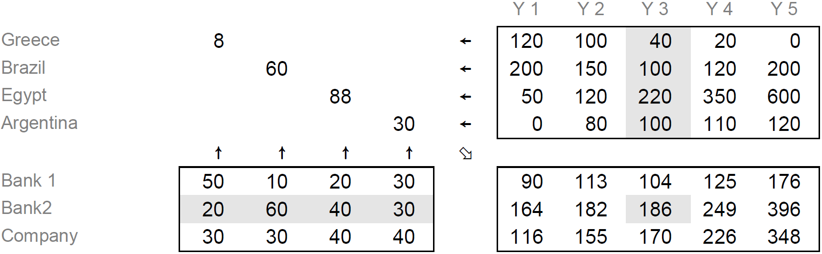
Fig. 11.2 Diagram representing the inner product operation.#
Fig. 11.2 has a great advantage: it clearly shows the relations that exist between the 3 matrices:
the left argument has as many columns as the right one has rows; and
the result has as many rows as the left argument and as many columns as the right one.
As you can see, the item result[x;y] is calculated from row x of the left argument (⍺[x;] in dfn notation) and column y of the right argument (⍵[;y] in dfn notation).
These rules will be generalised in the next section.
11.5.2. Definition of Inner Product#
The syntax of inner product is r ← x f.g y, where the inner product is represented by a dot (.) and f and g represent two appropriate dyadic functions (either primitive or user-defined).
The arguments may be arrays of any rank: scalars, vectors, matrices, or higher-rank arrays. The shape of the arguments and the shape of the result follow very simple rules:
the length of the last dimension of the left argument must be equal to the length of the first dimension of the right argument (in other words,
(¯1↑⍴x)≡1↑⍴y); andthe shape of the result is the catenation of the argugments’ shapes, in which the common dimension has disappeared (in other words,
(⍴r)≡(¯1↓⍴x),1↓⍴y).
Of course, as usual, scalars are repeated to fit the appropriate size.
Let us represent scalars by s, vectors by v, matrices by m, and higher-rank arrays by a.
The table below shows the same of the result of some inner products:
|
|
|
|
|---|---|---|---|
|
|
|
|
|
|
|
|
|
|
|
|
|
|
|
|
|
|
|
|
|
|
|
|
11.5.3. Typical Uses of Inner Products#
11.5.3.1. Two Simple Problems#
Many students imagine that matrix products are complex things, reserved for mathematicians, and far removed from everyday life. This opinion should be reconsidered: very simple problems can be solved using inner product.
hms is a variable which contains a time interval in hours, minutes, and seconds:
hms ← 3 44 29
We would like to convert it into seconds. We shall see three methods just now, and a fourth method will be given in another chapter.
A horrible solution:
(3600×hms[1]) + (60×hms[2]) + hms[3]
A good APL solution:
+/ 3600 60 1 × hms
An excellent solution with inner product:
3600 60 1 +.× hms
The second and third solutions are equivalent in terms of number of characters typed and similar in performance. However, it is recommended that you use the third one: it will help you become familiar with inner product so that after a certain period, it will become part of your toolkit as an APL programmer.
Here is a very similar example. Two vectors represent the prices of a certain number of goods and the quantities we bought:
price ← 6 4.2 1.5 8.9 31 18
qty   ← 2 6   3   5   1  0.5
To calculate how much we paid, we can use the beginner’s solution, or a solution with a simple inner product; they give the same result, of course:
+/ price × qty
price +.× qty
Just to show how it works, Fig. 11.3 contains an explanatory diagram similar to the one we used for our Banks/Investments example.
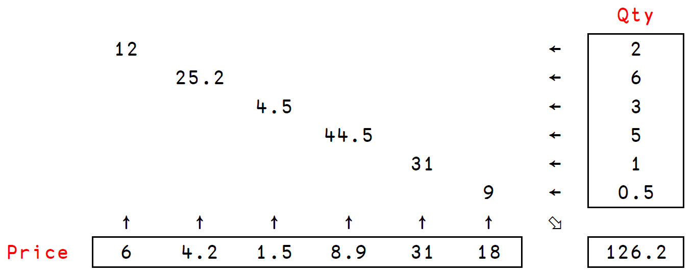
Fig. 11.3 Diagram explaining the behaviour of an inner product between two vectors#
11.5.3.2. A Useful Family#
Used with comparison functions, inner product offers 18 extremely useful derived functions.
Here is a vector ages containing the ages of 400 persons:
⎕RL ← 73
⎕← 20↑ages ← ?400⍴100  ⍝ We display the first 20 ages only.
In the same way as we did in Section 4.8.3, we can answer some elementary questions:
Are all these people younger than 65?
∧/ ages < 65
Is there at least one person younger than 20?
∨/ ages < 20
How many people are younger than 20?
+/ ages < 20
We can now replace reduce in the previous examples by inner product, like this:
Are all these people younger than 65?
ages ∧.< 65
Is there at least one person younger than 20?
ages ∨.< 20
How many people are younger than 20?
ages +.< 20
Clever, isn’t it?
These expressions can be read as:
∧.<means “all smaller” – are the ages all smaller than 65?∨.<means “at least one is smaller” – is there at least one age smaller than 20?+.<means “how many are smaller” – how many ages are smaller than 20?
In those three expressions, we have combined ∧, ∨, and + with <.
We could just as well combine them with all the comparison symbols, giving 18 different inner products, as shown in this table:
'∧∨+' ∘.{⍺,'.',⍵} '<≤=≥>≠'
11.5.3.3. A Special Case of a Comparison Inner Product#
In this family of inner products, ∧.= is particularly interesting, because it answers the question “are all those values equal?”.
For example, applied to vectors of the same length:
'customer' ∧.= 'customer'
'customer' ∧.= 'cucumber'
Let us use this property to search for a word in a matrix of words:
⎕← words ← 8 7⍴'CONTACTCOLUMNSFORTUNEPRODUCTCOLONELPROVIDEMACHINETYPICAL'
If we combine this 8 by 7 matrix with a 7-item vector, compatibility rules are obeyed, and the result will be a 8-item vector:
words ∧.= 'PRODUCT'
The shape of words is 8 7 and the shape of 'PRODUCT' is 7, so the common dimension disappears, and the result has shape 8.
Now, let us search for three words:
⎕← three ← 3 7⍴'MACHINECOMFORTPRODUCT'
words ∧.= ⍉three
We must transpose the matrix to be compliant with the compatibility rules, and the result shows what word was found in what row of words.
If we wanted to know which words were found, we could add an or-reduction:
∨⌿ words∧.=⍉three
If we wanted to know which of the rows in words contain words in three, we could have used another or-reduction, but along the other axis:
∨/ words∧.=⍉three
It may also be useful to search for the positions of said matches, but we can use index of for that:
words ⍳ three
The converse to the expression ∧.= is ∨.≠.
(That means that ∧.= and ∨.≠ always return opposite Boolean values.)
It looks for different values instead of looking for equal values.
Let us look at one simple example:
words ∨.≠ ⍉three
A 1 means that this word in three does not match the word in this row of words.
So, if a row contains all 1s, the word in that row does not match any of the words in three.
Using and-reduce along the second axis pinpoints the rows of words for which this is true:
∧/ words∨.≠⍉three
With a compression, we can see the words that are not found in three:
(∧/words∨.≠⍉three) ⌿ words
11.5.3.4. Similar Applications#
Very often it is desirable to find out whether any rows (or columns) of a matrix contain all blanks or all zeroes; or, alternatively, whether any rows or columns contain at least one non-zero number or a non-blank character.
To solve the first task we can use the same inner product as we used in most of the previous section (∧.=) and, to solve the second one, we can use the converse, which we introduced at the end of the previous section (∨.≠).
Suppose we have a matrix of characters mc and a matrix of numbers mn. Then,
mc ∧.= ' 'says which rows contain all blanks;mn ∧.= 0says which rows contain all zeroes;' ' ∧.= mcsays which columns contain all blanks;mc ∨.≠ ' 'says which rows contain at least one non-blank character;0 ∨.≠ mnsays which columns contain at least one non-zero number; and so on…
11.5.3.5. Shortest Routes in a Graph#
Finding the shortest routes in a graph is a classical problem to which inner product offers an elegant solution. Imagine 6 points in a town. They can be joined via a certain number of paths, according to Fig. 11.4.
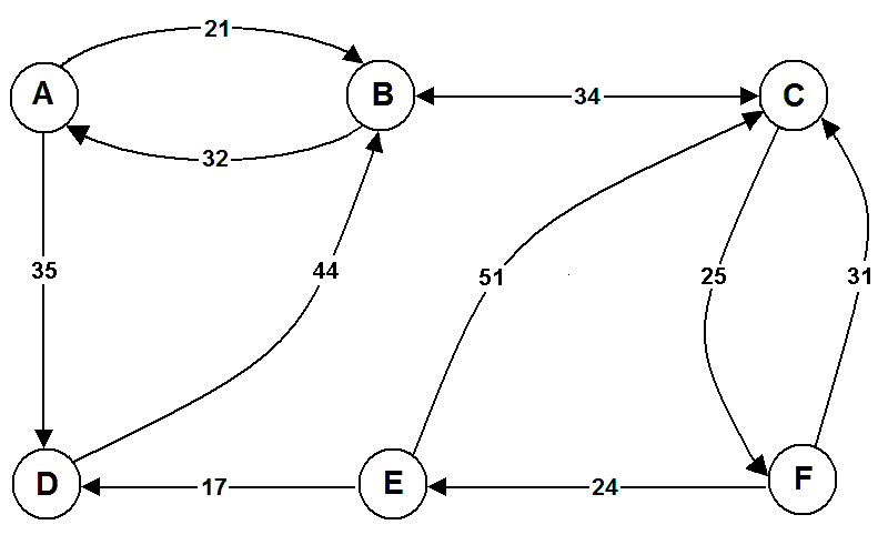
Fig. 11.4 A diagram with connections between 6 points in a town.#
We can create a matrix with the distances between the points.
The missing paths will be represented by a very high value (1000 in this case) to dissuade anyone from using them:
⍝ to            A    B    C    D    E    F
distances ←,    0   21 1000   35 1000 1000  ⍝ from A to ...
distances ,←   32    0   34 1000 1000 1000  ⍝ from B to ...
distances ,← 1000   34    0 1000 1000   25  ⍝ from C to ...
distances ,← 1000   44 1000    0 1000 1000  ⍝ from D to ...
distances ,← 1000 1000   51   17    0 1000  ⍝ from E to ...
distances ,← 1000 1000   31 1000   24    0  ⍝ from F to ...
⎕← distances ← 6 6⍴distances
The matrix distances contains distances from one point to another one, assuming we follow a single path.
The values 1000 indicate connections that cannot be made directly.
For example, there is no direct route from E to B; can we get there in two steps?
Let us consider all the possible pairs of routes from E to B:
Routes |
Distances |
Total distance |
|---|---|---|
|
1000 + 21 |
1021 |
|
1000 + 0 |
1000 |
|
51 + 34 |
85 |
|
17 + 44 |
61 |
|
0 + 1000 |
1000 |
|
1000 + 1000 |
2000 |
These computations could have been performed by APL.
The first set of distances considered refer to routes that start at E, which are the values of the fifth row of the matrix distances:
distances[5;]
Similarly, the second set of distances considered refer to routes that end at B, which are the values of the second column of the matrix distances:
distances[;2]
Therefore, all we have to do is sum the fifth row “from E” to the second column “to B” and we get distances of paths from E, with a possible intermediate stop, that end at B:
distances[5;] + distances[;2]
Only two routes really exist, because they are smaller than 1000, which are the ones of length 85 and 61.
Of course, we shall choose the shortest one:
⌊/ distances[5;]+distances[;2]
To obtain all the minimum routes that have one or two steps, we just have to repeat this calculation for all rows and columns: an inner product by the minimum of sums will do that.
⎕← L2 ← distances ⌊.+ distances
This result shows new routes, for example from A to C, from B to F, and others.
The matrix distances contains zeroes in the diagonal, because the distance from a point to itself is zero.
That means that the inner product computed above shows a matrix that displays the length of the shortest route between two points that makes use of one or two roads.
That is why the matrix was called L2.
Notice that L2 and distances have some common values:
L2 = distances
That is because the matrix distances already tells us what are the shortest routes between two points that make use of a single road.
Typically, going directly from a starting point to your final destination is faster than going through an intermediate stop, and that is why many values in L2 match distances.
If we compute yet another inner product, we determine the lengths of the shortest routes between two points that make use of one, two, or three roads:
⎕← L3 ← L2 ⌊.+ distances
Again, L3 and L2 have some values in common:
L3 = L2
The values in common refer to connections for which considering a third road doesn’t help.
For example, you couldn’t go from A → C directly, but if you go through B, then you can go from A → B → C, and the length of that path is 55.
When computing L3, we try to see if there is a path A → C, using three roads, that is faster than the path we already know.
For example, is the path A → D → B → C faster?
In this case, it isn’t, and that is why L3[1;3] and L2[1;3] are the same:
L3[1;3] = L2[1;3]
Imagine, however, that better roads are built in the directions A → D and D → B:
newDists ← distances
newDists[(1 4)(4 2)] ← 5 5
⎕← newDists
Now, using one or two roads, you can go from A to C in:
(newDists ⌊.+ newDists)[1;3]
However, if we consider routes that use one, two, or three roads, we can make use of the new better roads and go from A to C faster:
(newDists ⌊.+ newDists ⌊.+ newDists)[1;3]
If we ignore these new roads and continue using the distances we saw before, we can do one final inner product between L3 and distances to figure out how to connect all points:
⎕← L4 ← L3 ⌊.+ distances
L4 does not contain the value 1000, so we see it is possible to go from any point to any point using four roads or less.
If we tried doing an additional inner product, we would see that all values would stay the same, which means we already know the shortest routes possible:
L4 ≡ L4 ⌊.+ distances
Here is a representation of all the connections:
' ABCDEF','ABCDEF'⍪L4
These computations using inner product are elegant, but they have a shortcoming:
we found, for example, that the shortest path from D to E has length 127, and that it requires four steps, but we do not know which ones those four steps are.
11.5.3.6. Is a Graph Connected?#
In some development projects involving large graphs, it is sometimes necessary to check whether all points can be reached from any other point. In our town analogy from before, this would amount to checking whether we could go from any location to any other location, regardless of the length of the route.
We already know the answer for the diagram in Fig. 11.4, so let us consider a modified version in Fig. 11.5:
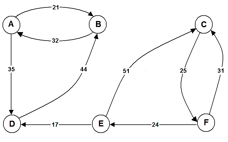
Fig. 11.5 A modified diagram with connections between 6 points.#
To check if the graph is connected (to check if you can go from any point to any other point), we can represent connections with a 1 and absence of connections with a 0:
connections ←, 1 1 0 1 0 0
connections ,← 1 1 0 0 0 0
connections ,← 0 0 1 0 0 1
connections ,← 0 1 0 1 0 0
connections ,← 0 0 1 1 1 0
connections ,← 0 0 1 0 1 1
connections ← 6 6⍴connections
' ABCDEF','ABCDEF'⍪connections
In the matrix distances, the diagonal was set to 0 because the distance from a point to itself was 0.
In the matrix connections, the diagonal is set to 1 because each point is (obviously!) connected to itself.
The matrix connections determines the direct connections between points, and we can see there is no direct connection from C to E:
connections[3;5]
Is there a connection in two steps?
This connection will exist if we can go from C to A and from A to E, or from C to B and from B to E, or … and so on.
Repeated for all points, this connectivity matrix in two steps can be obtained using an inner product by or and and:
⎕← C2 ← connections ∨.∧ connections
Now, we can see that C is connected to E:
C2[3;5]
We can keep computing these inner products:
⎕← C3 ← C2 ∨.∧ connections
⎕← C4 ← C3 ∨.∧ connections
⎕← C5 ← C4 ∨.∧ connections
The matrix C5 tells what points are connected by routes with 5 steps or less.
Do we need to compute another inner product?
Our town has 6 different points of interest. If you cannot go from one place to another in 5 steps, there is no point in trying 6 steps: routes with 6 steps will mean we are repeating intermediate stops, which does not help in trying to reach a specific destination.
So, our final connectivity matrix is C5:
C5
Because it contains 0s, it shows that we cannot go from D to C, for example.
You can confirm this by looking at Fig. 11.5 and realising there is, indeed, no roads that take us from D to C.
11.5.4. Other Uses of Inner Product#
We saw above some common uses of inner product, but there are many other useful inner products using primitives or even user-defined functions. Learning to recognise patterns where an inner product is applicable is just a matter of practice.
As for outer product, some applications of inner product produce nested arrays, as you can see with the following examples:
⎕← a ← 2 3⍴2 4 1 1 3 5
⎕← b ← 3 4⍴3 0 2 5 1 7 7 2 6 0 4 2
a ,.+ b
a +., b
11.5.5. Application#
We have a certain number of two-dimensional points, the coordinates of which are given by a nested vector:
⍝ points:    A     B     C     D      E     F     G    H
coords ← (0 2)(¯1 2)(¯2 1)(¯1 0)(¯1 ¯1)(1 ¯3)(2 ¯2)(2 0)
Now, we take those coordinates and then split them into vectors with the x and y coordinates:
⎕← (x y) ← ↓[1]↑coords
Fig. 11.6 shows where those points are located in a coordinate system, and the polygon we get when we connect those points:
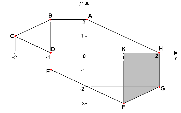
Fig. 11.6 A polygon with eight vertices.#
The area of the polygon can be calculated by adding the areas of the trapeziums delimited by the polygon and the horizontal axis, like the grey trapezium \([FGHK]\).
For each of those trapeziums, their base lengths are calculated by subtracting adjacent values in x:
x - 1⌽x
Then, the base lengths have to be multiplied by half of the sums of adjacent values in y:
(y + 1⌽y)÷2
In other words, we must add the products of bases by heights, which can be written as an inner product:
(x-1⌽x) +.× (y+1⌽y)÷2
What about the perimeter now? We must add all the individual segment lengths. The length of a segment \([BC]\) or \([FG]\) can be calculated using the Pythagorean theorem: \(a^2 + b^2 = c^2\).
We shall calculate the length of horizontal and vertical sides by subtracting adjacent values in x and y, as we did for x in the previous example.
⎕← segs ← (x-1⌽x),[1.5](y-1⌽y)
Now, in each small right-angled triangle, we must add the squares of both sides to obtain the square of each hypotenuse: add the squares will be our first inner product:
segs +.* 2
Then, we have to add the square roots of these hypotenuses. Add the square roots will be our second inner product:
(segs +.* 2) +.* 0.5

11.6. Intermission Exercises#
Exercise 11.2
You are given the matrix mat shown below.
Calculate the result of the following expressions and then check your answers on the computer:
⌈/ mat⌊/ +/ mat×/ ⌊/[1] mat×/ ⍴mat
mat ← 3 5⍴8 2 5 1 4 3 7 1 5 0 4 3 6 0 6
Exercise 11.3
Calculate:
-\ 6⍴1-\ ⌽⍳5×/ +\ 6⍴1
Exercise 11.4
Calculate:
∧/ 1 1 1 0 1 1∧\ 1 1 1 0 1 1=/ 0 1 1 1 0 1 1=\ 0 1 1 1 0 1 1
Exercise 11.5
When we execute ×\vec, we get the result 7 14 70 210 840.
What is the value of vec?
Exercise 11.6
Broken keyboard!
The iota (⍳) key of your keyboard does not work.
How could you create the list of the first n integers?
Exercise 11.7
Let \(a\), \(b\), and \(c\), be the three sides of a triangle, and \(s\) be its semi-perimeter (half of its perimeter, \(s = \frac{a + b + c}2\)). Believe it or not, the area of that triangle is equal to the following expression (called “Heron’s formula”):
Can you write a function to calculate the area of a triangle given the lengths of its sides? Use the two examples below to validate your solution.
Area 3 4 5
VALUE ERROR: Undefined name: Area
      Area 3 4 5
      ∧
Area 10 6 8
VALUE ERROR: Undefined name: Area
      Area 10 6 8
      ∧
Exercise 11.8
We would like to know whether all the items of a vector are different.
Among the many possible solutions, could you find one using outer product and another one using inner product?
The result must, of course, be a Boolean 0 or 1.
Exercise 11.9
What would be the result of 2 =/ 'MASSACHUSSETTS'?
Exercise 11.10
Try to find a word in a vector of characters. Your function should give the positions of the first letter of the word in the vector.
After solving this exercise once, try to also implement this function In using an inner product.
Solving the next two exercises first might help.
'CAN' In 'CAN YOU CANCEL MY FLIGHT ON AIR CANADA?'
VALUE ERROR: Undefined name: In
      'CAN'In'CAN YOU CANCEL MY FLIGHT ON AIR CANADA?'
           ∧
Exercise 11.11
Broken keyboard!
Try to find a row in a matrix without using dyadic iota ⍳.
Your function InMat should expect a matrix on the left and a vector on the right, and it should return a Boolean value indicating whether the left argument matrix contains a row equal to the right argument vector.
You can assume the matrix has as many columns as the vector has elements.
(4 3⍴'BANCANDANDIG') InMat 'CAN'
VALUE ERROR: Undefined name: InMat
      (4 3⍴'BANCANDANDIG')InMat'CAN'
                          ∧
(4 3⍴⍳12) InMat 0 1 2
VALUE ERROR: Undefined name: InMat
      (4 3⍴⍳12)InMat 0 1 2
               ∧
Exercise 11.12
Modify the previous exercise so that the right argument can either be a vector or a matrix. Your function should return a vector with as many elements as there are rows on the right argument (or with one element, if the right argument is a vector), where each element is a Boolean value indicating whether the corresponding row of the right argument matches any of the rows of the left argument matrix.
Can you use inner product in this exercise and/or in the previous one?
(4 3⍴'BANCANDANDIG') InMat2 'CAN'
VALUE ERROR: Undefined name: InMat2
      (4 3⍴'BANCANDANDIG')InMat2'CAN'
                          ∧
(3 3⍴9 8 7 4 5 6 3 2 1) InMat2 2 3⍴⍳6
VALUE ERROR: Undefined name: InMat2
      (3 3⍴9 8 7 4 5 6 3 2 1)InMat2 2 3⍴⍳6
                             ∧
Exercise 11.13
For a certain number of people, you are given two vectors:
status– a character vector specifying the person’s marital status (Single, Married, Divorced, Widow, Unknown); andgraduated– a character vector specifying if the person has graduated or not (Yes/No).
Write a function to count how many people are in each category.
CrossCount ← {binx ← (∪⍺)∘.=⍺ ⋄ biny ← ⍵∘.=(∪⍵) ⋄ r ← binx +.∧ biny ⋄ ((⊂''),(⊂'Total'),⍨∪⍵)⍪((⊂'Total'),⍨∪⍺),(⊢⍪+⌿)(⊢,+/)r}
⎕RL ← 73
⎕← 10↑status ← 'SMDWU'[?300⍴5]
⎕RL ← 73
⎕← 10↑graduated ← 'YN'[?300⍴2]
graduated CrossCount status
11.7. At#
The operator at can be used to work with values at specified positions, and there are multiple ways in which we can do this. In its most general form, the operator at can work with right arguments of arbitrary rank, but for the sake of simplicity we will start by explaining how the operator works with vectors as right arguments.
11.7.1. Apply Function At Indices#
In one of its forms, the operator at can be used to apply a function at the specified indices of the argument vector. The function to be applied is the left operand and the indices are the right operand.
This is the first time we learn about an operator that takes an array as the right operand. In the example below, notice how we use parentheses to separate the right operand array from the right argument array.
Let us negate the values at indices 1, 3, and 9, of vector:
vector ← 10×⍳10
idx ← 1 3 9
(-@idx) vector
Notice that the operator at returns the whole array after modifying the specified values, in opposition to returning just the values that were modified.
The parentheses around -@idx are necessary.
If they were not there, APL would not complain, but it would produce some interesting output:
-@idx vector
What is happening is that APL is looking at idx vector as a vector of length two defined by strand notation.
We can verify that idx vector is being interpreted as a single array.
We do that by parenthesising idx vector and noticing that the interesting output does not change:
-@(idx vector)
The exact meaning of this output will be explained in Section 12.2.
For now, it suffices to understand that it does not the output of (-@idx) vector.
In order for APL to know that idx is the right operand and vector is the right argument, we must separate them in some way.
Parenthesising the operator and its operand is one option, but another common option is to just use a right tack:
-@idx ⊢ vector
The right tack works because it effectively breaks the strand, which lets the operator at understand that its right operand is just idx.
Below, you can find another example usage of the operator at, in which we double values at the indices 1 and 10 with a dfn:
{⍵×2}@1 10⊢ vector
The example above also shows that the operator at works with user-defined functions.
It is important to understand how the operator at passes the elements of the indices specified into the left operand function. Take a look at the definition of the nested vector below:
⎕← nested ← ⍳¨⍳5
What is the output you expect from running the expression (⍴@4 5)nested?
Give it some thought…
Because the actual result might surprise you:
⍴@4 5⊢nested
The operator at collects all the elements at the indices specified and then passes them, as a whole vector, to the left operand function. We can see this by using, as the left operand, a dfn that prints its right argument:
_ ← {⎕←'called with ⍵: ' ⋄ ⎕←⍵ ⋄ ⍵}@4 5⊢nested
This is different from passing each element to the left operand function separately when the left operand function is not a scalar function, like ⍴.
Then, after all the values are collected and passed in to the left operand function, the result should be a single scalar (that gets placed in all the indices specified) or a vector with as many elements as there were indices. In that case, the elements of the result vector are distributed across the positions specified by the indices.
The example above with shape at and the nested vector shows that a scalar result gets placed in all the positions that were specified. The example below shows that the result vector must have as many elements as there were indices, otherwise the operator at will not know how to place the results:
⎕← matrices ← {⍵ ⍵⍴⍳⍵*2}¨⍳3
⍴@3⊢matrices
LENGTH ERROR
      ⍴@3⊢matrices
      ∧
The reason we get a LENGTH ERROR above is that the shape at index 3 returns 3 3, which is a vector of length 2, which does not match the length 1 of the vector of indices.
11.7.2. Apply Dyadic Function At Indices#
When the function in (F@idx)vector is dyadic, the left argument of F can be written on the left of the operator at, as left (F@idx) vector.
In this case, the operator at does not do any sort of selection or indexing into the left argument.
The left argument is passed directly to the function F:
10 100 ×@3 5 ⊢ vector
Thus, if the function F is a scalar function, the left argument must be a scalar or have the same length as the vector of indices:
10 100 1000 ×@3 5 ⊢ vector
LENGTH ERROR: Mismatched left and right argument shapes
      10 100 1000×@3 5⊢vector
                 ∧
100 ×@1 3 5 ⊢ vector
11.7.3. Replace Values At Indices#
Here is the nested vector from before:
nested
Can you use a dfn to replace the elements of nested at indices 3 and 5 with the vectors 'CAT' and 'DOG', respectively?
There are a couple of ways to do this. For example, we can set the left operand to be a function that returns the left argument, and pass the new values as the left argument:
'CAT' 'DOG'{⍺}@3 5⊢nested
This is equivalent to just enclosing the new values in a dfn in the left operand:
{'CAT' 'DOG'}@3 5⊢nested
The operator at can, indeed, be used to replace values at the specified indices. We used a couple of different functions to do that, but the operator at provides a special form, in which the left operand is an array instead of a function.
Suppose we have a vector vec and a vector with some indices, idx.
If the vector new has the same length as idx, then we have seen that ({new}@idx)vec puts the elements of the vector new in the positions specified by the indices idx, but we can actually do this more directly by writing (new@idx)vec.
That is, the operator at can take a vector on the left, instead of a function, and it will put those values in the positions specified:
'CAT' 'DOG'@3 5⊢nested
The operator at has another form that we discuss next.
11.7.4. Right Operand as Selector#
So far, the forms we have seen with the operator at had an array right operand (more specifically, a vector). The operator at can also take a right operand selector function. This function must return a Boolean mask that determines to which values the left operand is applied.
For example, the code below replaces all values larger than 5 with the value 0:
⎕← vector ← 10?10
IsLarger5 ← {⍵>5}
0@IsLarger5⊢ vector
When the right operand is a function, that function must be prepared to receive the whole right argument array at once. In other words, the selector function is not applied individually to each element of the right argument.
So, if we define LongerThan3:
LongerThan3 ← {3<≢⍵}
And if we recall the vector nested:
nested
We might have expected ({3↑⍵}@LongerThan3) nested to trim the two last vectors.
Instead, it raises an error:
{3↑⍵}@LongerThan3⊢ nested
RANK ERROR: Right operand and argument ranks differ
      {3↑⍵}@LongerThan3⊢nested
           ∧
The error happens because LongerThan3 takes the whole vector nested as its argument and produces a scalar result, the Boolean value 1:
LongerThan3 nested
Then, the operator at sees that result as the Boolean mask that will determine what values get passed in to the left operand function.
However, the Boolean mask is just a scalar 1 and the right argument is a vector, so there is a rank mismatch and the operator at cannot do its magic.
If we modify the function LongerThan3 to return its result as a vector, we would still have an error, but this time a LENGTH ERROR:
LongerThan3 ← {,3<≢⍵}
{3↑⍵}@LongerThan3⊢ nested
LENGTH ERROR: Right operand and argument lengths differ
      {3↑⍵}@LongerThan3⊢nested
           ∧
This time, the error is a LENGTH ERROR because the Boolean mask is the vector ,1 which has length 1, whereas the argument vector nested has length 5.
As we have seen, the operator at is very versatile. As a right operand, you can have:
the set of indices where you want to do some work; or
a selector function that produces a Boolean mask indicating the positions where you will do some work.
As a left operand, you can have:
a function to be applied to the subarray that was selected; or
new values to replace the subarray that was selected.
The left operand acts on the selection of the right operand.
11.7.5. At with High-Rank Arguments#
So far, all of our examples with the operator at were with vectors. However, the operator at can handle right arguments of arbitrary rank. We just need to understand how those high-rank arrays are handled by the operands of the operator at.
11.7.5.1. Right Operand Array#
The right operand array can be a simple integer vector or a nested integer vector. If it is a simple integer vector (or a simple integer scalar), then the integers are the indices of major cells of the argument.
For example, we can easily increment the second and fourth rows of a matrix:
⎕← mat ← 4 4⍴⍳16
1000 +@2 4⊢ mat
If the right operand is nested, it specifies indices for reach or choose indexing.
For example, below we negate the four corners of our matrix mat:
-@((1 1)(1 4)(4 1)(4 4))⊢mat
11.7.5.2. Right Operand Function#
When the right operand is a function, it must still compute a Boolean mask that determines what values will be modified or replaced.
For example, we can easily add one to the odd values in the matrix:
1 +@{2|⍵} mat
11.7.5.3. Shape of the Left Operand#
So far, all the examples that we saw and that involved high-rank arrays avoided the issue of shapes:
If the left operand is a function, what will be the shape of its argument?
If the left operand is an array, what should its shape be for at to know how to replace the values?
Before you proceed and read this section, try to do some experiments to see if you can deduce these rules on your own.
Ready?
If the right operand is an array that specifies indices and the left operand is an array of replacement values, then the shape of the left operand must conform to the shape induced by the right operand.
If the right operand is an integer vector specifying major cells, the left operand must be of the same rank as the right argument, and it must have as many major cells as the length of the right operand:
(100+3 4⍴⍳4)@2 3 4⊢mat ⍝ 3 indices, left operand has 3 rows.
If the right operand is a nested array that uses reach or choose indexing to select which values will be replaced, then the left operand must have the same shape as the array of indices:
corners ← (1 1)(1 4)(4 1)(4 4)
(⍳4)@corners⊢mat ⍝ vector ←→ vector
(2 1 2⍴⍳4)@(2 1 2⍴corners)⊢mat ⍝ 2 1 2 cuboid ←→ 2 1 2 cuboid
If the right operand is an array that specifies indices and the left operand is a function, then the right argument of the function will have the shape induced by the right operand (as seen in the previous case) and it must return an array of the same shape.
If we use choose indexing with a two by two matrix to select the corners of our matrix mat, then the right argument of the left operand will be a two by two matrix and so must be the return value:
{⎕←'right arg:'⍵ ⋄ 2 2⍴⍳4}@(2 2⍴corners)⊢mat
Similarly, if we use a simple integer vector vec to select major cells of array, the right argument of the left operand will have shape equal to (⍴vec),1↓⍴array and the return value should have the same shape:
{⎕←'shape:'(⍴⍵) ⋄ 2 4⍴⍳4}@(2 3)⊢mat
If the right operand is a function that computes a Boolean mask, the values that are selected will be ravelled into a vector.
If the left operand is a replacement array, such an array must be a vector with the same length as the ravel of the selected values.
If the left operand is a function, its right argument will be the ravel of the values selected and it must return a vector with the same length.
The only exception to these two bullet points is if the left operand array is a scalar or if the left operand function returns a scalar. In that case, all the values selected will be replaced by that scalar.
Let us demonstrate these rules by using the operator at on the matrix mat:
mat
We will be working on the central two by two region of the matrix:
mat ∊ 6 7 10 11
We can replace those four values with four other values, if those are in a vector:
(100×⍳4)@{⍵∊6 7 10 11}mat
We can transform those four values, as long as the left operand returns a vector of length four:
{1⌽⍵}@{⍵∊6 7 10 11}mat ⍝ transform those 4 values
The left operand can also be, or return, a scalar. In that case, the scalar will replace all the selected values:
0@{⍵∊6 7 10 11}mat ⍝ replace all with 0
11.8. Rank Operator#
The operator rank is represented by the character jot diaeresis ⍤, and you can type it with the keys APL+Shift+J.
A good mnemonic is that it is the jot (APL+j) with something on top (Shift).
The operator rank is a powerful operator that allows you to apply functions to sub-arrays of your argument arrays.
The function to be applied is the left operand F and the sub-arrays to which F is applied are defined by the right operand spec.
11.8.1. Sub-Arrays in the Monadic Case#
Typically, the best way of helping new learners grasp how the operator rank works is by exploring the result of ⊂⍤spec for various integer scalars spec and for the case where ⊂⍤spec is used monadically.
With that in mind, we define a cuboid below:
⎕← cuboid ← 2 3 4⍴⍳24
The operator rank in ⊂⍤spec ⊢ cuboid will apply the function enclose to the cells of cuboid that have rank specified by spec:
if
specis0, the operator rank will enclose all the scalars in the cuboid because scalars have rank0;if
specis1, the operator rank will enclose all the rows of the cuboid because rows have rank1;if
specis2, the operator rank will enclose all the planes / sub-matrices in the cuboid because planes have rank2; andif
specis3or more, the operator rank will enclose the whole cuboid because the cuboid has rank3.
⊂⍤3⊢cuboid
⊂⍤2⊢cuboid
⊂⍤1⊢cuboid
⊂⍤0⊢cuboid
As these examples show, the operator rank led the function enclose (its left operand) to the sub-arrays that had the rank that was chosen by the right operand.
Suppose that we wanted to transpose each of the two sub-matrices of the cuboid. One can achieve that effect with dyadic transpose, but we can also look at that as transpose rank 2, which means we transpose the cells that have rank 2:
⍉⍤2⊢cuboid
11.8.2. Sub-Arrays in the Dyadic Case#
The derived function of the operator rank can also be used dyadically. In that case, the operator rank will pair up sub-arrays of the left argument with sub-arrays of the right argument. The sub-arrays of both sides do not have to be of the same rank.
In general, the dyadic case looks like left (F⍤i j) right.
The integer scalar i determines the rank of the sub-arrays of the left argument left and the integer scalar j determines the rank of the sub-arrays of the right argument right.
In order for the operator rank to be able to pair up sub-arrays of the left argument with sub-arrays of the right argument, there has to be some shape compatibility: the frames of the left and right argument must be the same. The frames are composed of the leading axes of the arguments that are not included in the sub-arrays:
the frame of the left argument is
fl ← (-i)↓⍴left; andthe frame of the right argument is
fr ← (-j)↓⍴right.
So, left F⍤i j ⊢ right only works if fl ≡ fr, that is, if ((-i)↓⍴left)≡((-j)↓⍴right).
For example, suppose left has rank 5 and shape 2 3 4 5 6 and right has rank 4 and shape 2 4 3 8:
left ← 2 3 4 5 6⍴0
right ← 2 4 3 8⍴0
the expression
left F⍤4 3 ⊢ rightis a valid usage of the operator rank because:the frame of
leftis2, which is¯4↓⍴left; andthe frame of
rightis also2, which is¯3↓⍴right.
_← left {⍺ ⍵}⍤4 3 ⊢ right ⍝ works without error
the expression
left F⍤4 2 ⊢ rightdoes not work and gives aRANK ERRORbecause the frames of the left and right arguments do not have the same rank:the frame of
leftis2, which is¯4↓⍴left; andthe frame of
rightis2 4, which is¯3↓⍴right.
_← left {⍺ ⍵}⍤4 2 ⊢ right ⍝ RANK ERROR
RANK ERROR
      _←left{⍺ ⍵}⍤4 2⊢right  ⍝ RANK ERROR
                 ∧
the expression
left F⍤3 2 ⊢ rightdoes not work and gives aLENGTH ERRORbecause the frames of the left and right arguments do not have the same axes lengths:the frame of
leftis2 3, which is¯3↓⍴left; andthe frame of
rightis2 4, which is¯2↓⍴right.
_← left {⍺ ⍵}⍤3 2 ⊢ right ⍝ LENGTH ERROR
LENGTH ERROR: It must be that either the left and right frames match or one of them has length 0
      _←left{⍺ ⍵}⍤3 2⊢right  ⍝ LENGTH ERROR
                 ∧
The error message above shows one more situation in which the operator rank works. If the sub-arrays of the left argument match the whole left argument or if the sub-arrays of the right argument match the whole right argument, then the operator rank will pair that argument with all the sub-arrays of the other argument.
the expression
left F⍤5 j ⊢ rightworks for any value ofjbecause the frame ofleftis⍬and therefore has length zero.
_← left {⍺ ⍵}⍤5 0 ⊢ right  ⍝ works!
_← left {⍺ ⍵}⍤5 1 ⊢ right  ⍝ works!!
_← left {⍺ ⍵}⍤5 2 ⊢ right  ⍝ works!!!
_← left {⍺ ⍵}⍤5 3 ⊢ right  ⍝ works!!!!
Similarly,
the expression
left F⍤i 4 ⊢ rightworks for any value ofibecause the frame ofrightis⍬and therefore has length zero.
_← left {⍺ ⍵}⍤0 4 ⊢ right  ⍝ works!
_← left {⍺ ⍵}⍤1 4 ⊢ right  ⍝ works!!
_← left {⍺ ⍵}⍤2 4 ⊢ right  ⍝ works!!!
_← left {⍺ ⍵}⍤3 4 ⊢ right  ⍝ works!!!!
_← left {⍺ ⍵}⍤4 4 ⊢ right  ⍝ works!!!!!
To illustrate better how the pairing of the operator rank works, we can consider the dfn {⍺ ⍵} that will strand the left and right sub-arrays.
First, we will pair all sub-matrices on the left with all scalars on the right.
(3 4 5⍴⎕A) {⍺ ⍵}⍤2 0 ⊢ ⍳3
Now, we will pair all rows on the left with the right argument vector.
(3 4 5⍴⎕A) {⍺ ⍵}⍤1 1 ⊢ ⍳3
Notice how, in the example above, the right argument vector was repeated 12 times, one for each of the sub-arrays of the left argument.
11.8.3. Cells#
The sub-arrays of rank r of an array are typically referred to as r-cells of that array.
0-cells are scalars;1-cells are vectors and sometimes referred to as rows;2-cells are matrices and sometimes referred to as planes or tables;…
So, the expression F⍤k ⊢ array can be said to apply F to the k-cells of array.
We can say the same thing the other way around: the k-cells of array are its sub-arrays on the last k axes.
11.8.3.1. Negative k#
If k is negative, a k-cell of an array of rank r is the same as a r+k-cell.
Using negative values of k can be advantageous because this makes it so that the actual rank of the cell depends on the rank of the original array.
For example, a ¯2-cell on a matrix is actually a (2+¯2)-cell (a scalar), and a ¯2-cell on a cuboid is actually a (3+¯1)-cell (a vector).
11.8.3.2. Major Cells#
¯1-cells are commonly referred to as major cells because they are the largest cells of an array, as far as rank is considered.
Below, you can find a table with common arrays and the corresponding major cells.
Array |
Major cells are… |
|---|---|
vector |
scalars |
matrix |
vectors |
cuboid |
matrices |
4D array |
cuboids |
11.8.4. Specifying Cells#
Now that we are aware of what cells are, the operator rank can actually be defined in terms of cells of the left and right arguments.
The expression F⍤k ⊢ right will apply the function F monadically to the k-cells of right and the expression left F⍤i j ⊢ right will apply the function F dyadically between the i-cells of left and the j-cells of right.
In particular, the operator rank can deal with cell specifications that have negative numbers.
For example, the expression ⊂⍤¯1 turns any array into a vector of its major cells.
If we have a matrix:
3 3⍴⍳9
we get a vector of its rows:
⊂⍤¯1 ⊢ 3 3⍴⍳9
And if we have a cuboid:
2 3 4⍴⍳24
we get a vector of its sub-matrices:
⊂⍤¯1 ⊢ 2 3 4⍴⍳24
The operator rank has another form that contemplates the monadic and dyadic uses of the derived function in one single cell specification, but we will only cover it in Section 11.15.4.
11.9. Key#
The operator key is represented by the glyph ⌸ and you can type it with APL+Shift+K.
It is easy to remember the keyboard shortcut for key because key is in the letter K.
The operator key is monadic and its left operand must always be a dyadic function that returns a result.
The derived function can be used monadically or dyadically.
In both cases, the idea is that the operator key provides a way to group your values before applying F to each of those groups.
The expression groups F⌸ values will apply F to subsets of the major cells of values as defined by the major cells of groups.
Setting F ← {⍺ ⍵} and defining simple vectors for groups and values should bring some clarity to the way key works.
Let us define two vectors that contain the suits and values of some playing cards:
values ← '4' 'Jack' '6' 'Ace' '10'
suits ← 'Spades' 'Hearts' 'Spades' 'Clubs' 'Spades'
Now, we can group the cards by their suits:
suits {⍺ ⍵}⌸ values
As we can see, the function {⍺ ⍵} received, as left argument, each of the unique groups, also referred to as keys.
Its right argument was a vector with all the values that were associated with each key.
The monadic case F⌸ array is equivalent to the dyadic case array F⌸ ⍳≢array.
In other words, in the monadic case, the operator key uses the major cells of the argument as keys and then groups together the indices where each key appears:
{⍺ ⍵}⌸ 'MISSISSIPPI'
'MISSISSIPPI',[0.5]⍳11
11.9.1. Key with High-Rank Arguments#
The explanation above mentioned major cells and arrays in general because the operator key can be used with arrays of arbitrary rank as both arguments.
To showcase this ability, consider a matrix with names of some employees and the respective days they showed up for work:
⎕← employees ← ↑'ALICE' 'BOB' 'ALICE' 'BOB' 'CHARLES' 'ALICE' 'CHARLES'
dates ← '27/6' '27/6' '28/6' '29/6' '29/6' '30/6' '30/6'
We can group the employees by workday with the operator key:
dates {⍺ ⍵}⌸ employees
We can see that using a matrix as the right argument was not a problem.
What is more, we can see that because the right argument of {⍺ ⍵}⌸ had rank two, the right argument of the operand of key also receives arguments of rank two.
If the dates had been a 2-column matrix with day and month, key would still know how to group the employees:
⎕← datesMat ← 7 2⍴27 6 27 6 28 6 29 6 29 6 30 6 30 6
datesMat,employees
datesMat {⍺ ⍵}⌸ employees
In the example above, the operator key used the major cells of the left argument (its rows) to determine which keys to use. The left argument of the operand is always the key itself, so the left argument of the operand in the example above was the 2-element vector with the day and the month.
If we want to keep only the day of employment, since all records are relative to the month of June, we can extract it with ⊃⍺:
datesMat {(⊃⍺) ⍵}⌸ employees
11.9.2. Order of the Result#
The elements of the result of key appear in the same order as they appear in the argument vectors. This means that if the arguments are reordered, the result of applying key might also come in a different order:
{⍺ ⍵}⌸ 'MISSISSIPPI'
{⍺ ⍵}⌸ 2⌽'MISSISSIPPI'
The sub-sections that follow will cover a couple of common use-cases for the operator key.
11.9.3. Applications of Key#
11.9.3.1. Counting Unique Values#
One of the simplest and most common use cases for key is to count unique values in a vector, or unique major cells in any arbitrary array.
For example, we can quickly compute how many of each letter a word or sentence has:
{⍺(≢⍵)}⌸ 'MISSISSIPPI'
{⍺(≢⍵)}⌸ 'HOW ARE YOU DOING TODAY'
If you are counting occurrences of values of a predetermined number of categories, bear in mind that categories that are not represented will not show up with a zero in its count.
For example, we had some playing cards before:
values,⍪suits
None of the cards is of the suit diamonds, so when we count how many cards of each suit, we will not have a 'Diamonds' 0 in the result:
{(⊃⍺)(≢⍵)}⌸ suits
After all, the operator key cannot guess that the key 'Diamonds' was missing.
If you want all possible keys to show up, catenate them once to the argument array and then subtract one from the count.
If you catenate all the possible keys in the beginning, you can even force the order of the result:
allSuits ← 'Clubs' 'Diamonds' 'Hearts' 'Spades'
{(⊃⍺)(¯1+≢⍵)}⌸ allSuits,suits
Notice how the order of the vector allSuits was preserved in the rows of the result.
11.9.3.2. Summarising Data by Category#
The operator key can also be used to aggregate and summarise data by one or more keys. For example, suppose you have a log of purchases and sales of shares of different companies:
companies ← ↑'GOOG' 'MSFT' 'TSLA' 'MSFT' 'GOOG' 'GOOG' 'TSLA' 'GOOG' 'TSLA'
trades ← 100 120 80 ¯30 50 ¯100 ¯80 50 100
companies,trades
By using the operator key, we can easily aggregate the trades by company and then determine how many shares of each company we have:
companies {⍺(+/⍵)}⌸ trades
In this particular example, we used +/ to sum all of the trades that pertained to a single company.
This pattern of aggregating data and then summarising it works with every other summarising function you can think of.
For instance, if instead of trades we had data about the prices of the stock, we could easily determine what was the highest price each company attained:
companies ← ↑'TSLA' 'MSFT' 'GOOG' 'GOOG' 'GOOG' 'MSFT' 'TSLA' 'MSFT' 'TSLA'
prices ← 209.39 329.37 143.77 137.88 134.17 294.95 288.12 259.58 271.71
companies,prices
companies {⍺(⌈/⍵)}⌸ prices
11.10. Stencil#
11.10.1. Your First Stencil#
The operator stencil is represented by the glyph ⌺ and it is typed with APL+Shift+`.
Stencil ⌺ and the diamond ⋄ are in the same key, so use the fact that the stencil looks like a quad ⎕ around the diamond ⋄ as a mnemonic to know where stencil is.
The operator stencil is used to apply a function operand to rectangular sections of the argument array. The size and positioning of these rectangular sections is determined by the right operand of stencil and the left operand is the function that is applied to each section.
For example, we can have a 4 by 4 matrix and we can use the operator stencil to apply any given function to all its 3 by 3 sub-matrices. Before doing any computations with the sub-matrices, we can study how the operator stencil works and visualise what sub-matrices are created. To do that, we need to:
use the dfn
{⊂⍵}as the left operand, which will enclose each sub-matrix and allow us to visualise all of them;use the vector
3 3as the right operand, which will tell the operator stencil that we want sub-matrices that have shape3 3; anduse a matrix as the right argument to the derived function.
Here is an example:
⎕← mat ← 4 4⍴⍳16
{⊂⍵}⌺3 3⊢mat
Notice that some sub-matrices in the result above contain zeroes that were not present in the original matrix.
These rows and columns of zeroes are padding.
Padding is needed because the operator stencil creates sub-matrices centred on successive elements of the matrix mat.
However, you can only create a 3 by 3 matrix centred around 1 (the top-left number in mat) if you add a column of zeroes on the left of mat and a row of zeroes on the top of mat.
The result of using the operator stencil with the left operand {⊂⍵} can be intuitively described as the effect you get by placing a window of size 3 3 over the matrix mat, and then sliding that window over the matrix.
The padding is what you “see” when the window is slightly off the matrix.
11.10.2. Padding and Window Size#
As we have seen, the operator stencil sometimes adds padding to allow for the creation of sub-arrays centred on the successive elements of the argument array. However, the padding that is added depends on the size of the sub-arrays that are created, sometimes referred to as the size of the sliding window. If the sliding window is very big, the padding increases. If the sliding window is very small, the padding decreases.
The total padding added does not depend on the size of the argument array.
Below, we stick to the window size of 3 3 and use a larger matrix, and we see the padding remains the same:
{⊂⍵}⌺3 3⊢6 6⍴⍳36
With a window size of 3 3, the padding we get is still one row and one column around the matrix argument.
If we make the window size smaller, we get less padding. With a unit length window (the smallest window possible), we actually get absolutely no padding:
{⊂⍵}⌺1 1⊢6 6⍴⍳36
If we make the window larger, we get more padding:
{⊂⍵}⌺5 5⊢6 6⍴⍳36
The examples before all had an odd window size, but window sizes can also be even.
When the window size is odd, it is easier to see which number a window is centred on.
If the window size s is even, the central element is at the index s ÷ 2.
Let us use a window size of 4 and look at the very first sub-matrix of mat:
⊃ {⊂⍵}⌺4 4⊢mat
The window size is 4 4 and the first window is centred around 1, which is at index 2 2 of the sub-matrix:
(⊂2 2)⊃ ⊃ {⊂⍵}⌺4 4⊢mat
Let us look at all the sub-matrices:
{⊂⍵}⌺4 4⊢mat
When the window size is even, the padding we get seems to be the same as if the window size had been odd, and one less.
In this particular example, a window size 4 4 used the same padding as a window size 3 3.
In general, when the window size is even, the maximum amount of padding we see is one row/column less than half of the window size.
In the example above, the window size is 4 4, so the maximum padding we get is one less than half of that: half of that is 2 2 and one less is 1 1, so the maximum padding we get is one row and one column.
If we go back to the larger matrix, we can try having a window size of 6 6, to see that the maximum padding we get is 2 2:
⊃ {⊂⍵}⌺6 6⊢6 6⍴⍳36
The window does not have to be a square, so we can even pick different lengths for the number of rows and columns of each sub-matrix. As a result, the padding is also done independently for rows and columns.
We can split a matrix into sub-matrices that contain a single row and three columns, in which case there will be no padding added on top or on the bottom, but there will be padding on the left and on the right:
{⊂⍵}⌺1 3⊢mat
In its general form, if the window size is ws, then the padding you will get is ⌊(ws-1)÷2.
If we set ws to the example above:
ws ← 1 3
We get a confirmation that the padding was 0 1:
⌊(ws-1)÷2
11.10.3. The Left Operand Function#
The operator stencil takes a left operand function.
So far, we only used {⊂⍵} but that can be any dyadic function that returns a result.
The right argument of that function is the sub-array that the operator stencil computed and the left argument gives you padding information.
In fact, the left argument ⍺ is such that ⍺↓⍵ is a sub-array without padding.
In other words, the left argument of the left operand is the value you would need if you wanted to drop the padding from all sub-arrays.
Here are all the 3 by 3 sub-matrices of mat, with and without the padding that the operator stencil adds:
({⊂⍵}⌺3 3⊢mat)({⊂⍺↓⍵}⌺3 3⊢mat)
We can also try pairing the left and right arguments to see what ⍺ looks like:
{⊂⍺ ⍵}⌺3 3⊢mat
The definition of the left argument of the left operand also determines the maximum window size for any given array. Recall that the left argument is:
“the vector
⍺such that⍺↓⍵removes all padding from⍵.”
The primitive drop can drop from the beginning or end of any axis, but never from both ends at the same time.
For example, if you had the vector 0 0 1 2 3 0 you could drop all the zeroes in it by dropping two from the front and one from the back, but you always have to do that by using drop twice:
2↓¯1↓0 0 1 2 3 0
¯1↓2↓0 0 1 2 3 0
There is no left argument you can pass to drop that will let you get rid of the leading and trailing zeroes at the same time.
Thus, the maximum window size, is the window size that ensures there is never padding on both sides of a sub-array.
This is always 1+⍴array.
For example, here is a 3 by 7 matrix:
⎕← letters ← 3 7⍴⎕A
For this matrix, the maximum window size is:
1+⍴letters
Notice, however, that this maximum is per axis.
That is, a valid window size for the matrix letters must be less than or equal to 4 8 in each axis.
So, a window size ws is valid if ws ∧.≤ 4 8.
Conversely, a window size ws is invalid if ws ∨.> 4 8.
Here are some examples of invalid window sizes that raise DOMAIN ERROR:
ws ← 5 6
ws ∨.> 4 8
{⊂⍵}⌺ws⊢letters
DOMAIN ERROR
      {⊂⍵}⌺ws⊢letters
         ∧
ws ← 2 10
ws ∨.> 4 8
{⊂⍵}⌺ws⊢letters
DOMAIN ERROR
      {⊂⍵}⌺ws⊢letters
         ∧
ws ← 7 12
ws ∨.> 4 8
{⊂⍵}⌺ws⊢letters
DOMAIN ERROR
      {⊂⍵}⌺ws⊢letters
         ∧
Finally, here is the example that makes use of the largest possible window size:
{⊂⍵}⌺4 8⊢letters
Notice how the nested matrices in columns 3 and 4 contain the whole matrix letters, plus a row and a column of padding.
That shows that the padding is already at a maximum.
11.10.4. Stencil For Any Rank#
The operator stencil can be applied to arrays of any rank. The right operand array, which is responsible for determining the shape of the resulting sub-arrays, must contain as many elements as there are axes in the right argument.
In the examples above, we applied the operator stencil to matrices, which have rank two, which explains why the window size was always a vector with two integers. If we want to apply stencil to a vector (rank 1), then the right operand must have a single element:
{⊂⍵}⌺3⊢⍳10
And if we want to apply stencil to a cuboid (rank 3), then the right operand must have three elements:
{⊂⍵}⌺3 3 3⊢2 2 2⍴⍳24
11.10.5. Step Size#
The operator stencil defaults to creating all sub-matrices consecutively, but you can specify a step size that determines by how much the rectangular window moves. The step size is also indicated in the right operand, which in its most general form is a 2-row matrix:
the first row determines the window size along each axis; and
the second row determines the step size along each axis.
The first sub-array is always centred on the first element of the argument to stencil, so the step size only influences the subsequent sub-arrays that are created:
⎕← mat ← 3 3⍴⍳9
ws ← 3 3
The default step size is 1 on each axis:
stepSize ← 1 1
⎕← complete← {⊂⍵}⌺(2 2⍴ws,stepSize)⊢mat
The step size is specified independently for each axis, so we can increase the step size along the first axis to 2. This will skip every other row of sub-matrices:
stepSize ← 2 1
{⊂⍵}⌺(2 2⍴ws,stepSize)⊢mat
Notice how the two rows of the result above are the first and third rows of the nested matrix complete.
We can increase the step size even further, to 3.
With a step size of 3 for the first axis, we only get one out of every three rows of the output.
Because the matrix complete only has 3 rows, this means our result will have a single row (the first one):
stepSize ← 3 1
{⊂⍵}⌺(2 2⍴ws,stepSize)⊢mat
The step size can be increased arbitrarily, even if further increases do not modify the output:
{⊂⍵}⌺(2 2⍴ws,123409 1)⊢mat
A step size of 123409 along the first axis means that we keep one out of every 123409 rows. Because there are only 3 rows in the complete result, we keep the very first one, and that is it.
11.10.6. Image Processing with Stencil#
The operator stencil is very useful in domains like image processing or neural networks. A simple application example is the usage of the operator stencil to blur images.
Fig. 11.7 is an image we will blur:

Fig. 11.7 A screenshot of the Dyalog website in late 2022.#
Fig. 11.8 is the blurred version:

Fig. 11.8 A blurred screenshot of the Dyalog website in late 2022.#
The main piece of code that blurs the image is this:
Blur ← {(+⌿,⍵)÷49}⌺7 7
newImage ← Blur⍤2⊢image
The function Blur goes over sub-matrices of shape 7 by 7 and then computes the average value of each 7 by 7 sub-matrix as the new value that will go in a given position.
This is one way to achieve a simple blurring effect.
Then, the expression that computes the new image applies the function Blur to each 2-cell of the array image, because image is actually a cuboid with three layers, where each layer represents a colour channel in the RGB colour space.
(If you are not familiar with the RGB colour space, you can think of it as saying that a colour can be determined by its amount of red, green, and blue.
Thus, in our code, we need to blur the red, green, and blue, layers, which is why we use Blur⍤2.)
11.11. Power#
Power is a dyadic operator represented by the glyph ⍣ that you can type with APL+Shift+P, which is easy to remember because P is the initial letter of power and because the glyph ⍣ is just the * with a diaeresis on top.
The operator power produces a derived function that is either monadic, dyadic, or ambivalent, depending on the function used as the left operand.
Again, depending on the left operand, the derived function may return a result or not.
The general syntax is {result} ← {left} F⍣n ⊢ right, if the right operand is an integer, or {result} ← {left} F⍣C ⊢ right, if the right operand is a function.
The two usages are explained next.
11.11.1. Power n Times#
If the right operand n is an integer scalar, the left operand function F is applied n times to the argument right (if the derived function is used monadically) or to left and right (if the derived function is used dyadically).
Like with some other operators we have seen already, the right operand n must be separated from the right argument, either by parenthesising the whole derived function or by using a right tack between the right operand and the right argument.
Imagine we have a little matrix mat:
mat
And we write a function to spin it a quarter of a turn:
Spin ← {⊖⍉ ⍵}
Spin mat
Spin Spin mat
Of course, after 4 executions, the matrix would return to its original position.
We can spin the matrix any number of times using the operator power instead of writing Spin repeatedly:
Spin Spin mat
Spin⍣2⊢mat
Spin Spin Spin Spin Spin Spin Spin Spin Spin mat
Spin⍣9⊢mat
The example above shows that 9 spins are equivalent to a single spin.
The operator power can also give us a way of calculating a Fibonacci series:
Fibo ← {⍵,+/¯2↑⍵}
Fibo⍣10⊢1
11.11.2. Conditional Execution#
As a special case, when n is a Boolean value, the left operand function is applied (1) or not applied (0).
It simulates the conditional execution of the function.
In the example below, the right operand to power is 1, so we round down our values:
⌊⍣1 ⊢ 23.73 42.25
In the next example, the right operand to power is 0, so we do not round down:
⌊⍣0 ⊢ 23.73 42.25
For example, a function has been written in such a way that it works only on nested vectors, but sometimes its right argument v is a simple vector (not nested) or even a scalar.
So, one must ravel v (if it is a scalar), enclose it, then ravel again to produce a vector, or do absolutely nothing if v is already a nested vector.
The following expression will perform the necessary transformations: ({,⊂,⍵} ⍣ (1=≡,v)) v.
⎕← v ← 'nested' 'vector'
In this case, v is already a nested vector, so the expression above shouldn’t do anything to v:
({,⊂,⍵} ⍣ (1=≡,v)) v
In the next example, we define v to be a simple vector, which means the expression should nest it:
⎕← v ← 'simple vector'
⎕← newV ← ({,⊂,⍵} ⍣ (1=≡,v)) v
⍴newV
Whether one prefers to use the operator power to write such a compact conditional expression, or to use a traditional control structure (:If ... :EndIf) is mostly a matter of taste.
Some may find the former easier to write and read than the latter, while others may disagree.
The version with the operator power has the advantage that it works inside a dfn.
11.11.3. Left Argument#
If a left argument left is provided to the derived function, it is bound as the left argument to the left operand F in left F⍣n ⊢ right.
It is the same thing if, instead of an integer right operand, we have a function right operand in left F⍣C right.
So, the expression
3 ×⍣4⊢ 2
is the same as
  3× 3× 3× 3× 2
⍝ 1  2  3  4
and not
3 ×2 ×2 ×2 ×2
⍝ 1  2  3  4
11.11.4. Inverse Function#
If the right operand n is a negative integer, the function executed by the operator power is not F, but its inverse function – provided such an inverse function exists and APL knows about it.
If the inverse function to F is not known to APL, a DOMAIN ERROR will be reported.
In particular, APL is not able to find the inversion function of user-defined function, and some primitive functions have no inverse function.
If n is negative, the inverse function is applied |n times.
The function F may be an appropriate primitive function or an expression consisting of such primitive functions combined with primitive operators among each ¨, outer product ∘., axis [n], scan \, and power ⍣.
Later in Section 11.15.6 you will see that there are some other operators that you can also use and that the operator power will know how to invert.
As an example, let us compute the inverse of plus scan:
(+\ ⍣ ¯1) 3 4 9 15 19
We can confirm this result:
+\ 3 1 5 6 4
The inverse function can also accept a left argument:
left ← 2 5 3
⎕← right ← 3 4⍴10 4 14 8 25 10 35 20 15 6 21 12
left (∘.× ⍣ ¯1) right
In this case, the inverse function computed the vector that you would need to combine with the vector left to produce the matrix right:
right ≡ left ∘.× 5 2 7 4
11.11.5. Fixed Point and User-Defined Operators#
Here are two additional features of the operator power:
in its second form, the operator power has two function operands:
{left} F⍣C right; andsome common patterns in user-defined operators make use of power.
These two types of use require an advanced knowledge of APL and of user-defined operators. They will not be presented now, but Section 11.15.9 covers power with two function operands and Section 11.15.7 covers one such common pattern. Have a look at it when you feel ready.
11.12. Spawn#
11.12.1. Main Features#
The monadic operator spawn is represented by an ampersand & and your regular keyboard should be able to type it already.
It executes a function asynchronously from the main flow of execution in a separate sequence of instructions known as a thread.
If the main flow of execution and the function executing in the separate thread are both using the CPU heavily, nothing is gained by starting a separate thread. On the contrary, the two threads will be competing for the same resource – the CPU, which requires some overhead. But if one of the threads involves waiting time in which it cannot make use of the CPU, the other thread may use the CPU, which otherwise would have been idle. In such cases, a considerable improvement of the application’s perceived performance may be observed.
There are many situations in which a thread may be waiting and not be able to make good use of the CPU: it may be waiting for user input, a file operation, a response from a web client or server, or a response from a database manager, to give just a few examples.
Spawn is itself monadic, but its derived function is monadic, dyadic, or ambivalent, according to the definition of its left function operand. This function (and hence the derived function) may not be niladic.
Remark
If you are reading this book in its interactive format, we suggest you try the examples with the operator spawn in your local interpreter. That is because the operator spawn interacts in inconvenient ways with the notebook software.
Spawn returns as a shy result the number of the thread in which the task is executed.
The main execution flow is executing in thread number 0, so the first time one launches a new thread, it is executed in thread number 1.
Let us execute ⍳5 in a separate thread:
      ⎕← ⍳& 5
1
1 2 3 4 5
In the example above, the quad forces the shy result (the new thread number) to be displayed, which is 1 because this is the first thread we start. Then, the function result is displayed.
Remark
It may happen that you run the expression ⎕← ⍳& 5 and the output is the same as the one above, but with the two lines swapped.
If the left operand of spawn is a simple/small expression, it may finish executing before the quad gets a chance to print the thread number.
Once a thread number has been used, it will not be used again in this session: the thread number will be incremented every time spawn is used:
      ⎕← ÷& 2 5 10
2
0.5 0.2 0.1
As we can see, the second time we use spawn, the thread number was incremented to 2.
In these examples, the derived function was monadic; let us now use a dyadic function operand, and try to execute 2 3 7 × 4 6 5 in a separate thread:
      r ← 2 3 7 ×& 4 6 5
8 18 35
Beware of the previous example!
You may think that r contains the result of the function call, but it does not.
It contains the thread number:
      r
3
If you think about it, it should not come as a surprise that the result of starting a new thread is not the result of the function call. If that had been the case, the main execution thread would have had to stop and wait until the execution of the function had completed – and we would not have had any parallel execution at all!
So, if we cannot get hold of the result of the function call when starting it using the operator spawn, how can we get hold of it later, when we assume that the function has completed execution?
The answer is the monadic system function ⎕TSYNC (thread synchronization).
It takes an array of thread numbers as its argument.
It then causes the thread in which it is executing to stop and wait until all the threads listed in the argument have completed execution.
Then, it returns an array of the same shape as the right argument, each item containing the result of the function call executed in the corresponding thread.
Let us build a simple example using the system function ⎕DL (delay), which simply stops execution for approximately a specified number of seconds.
⎕DL returns, as a result, the exact length of the delay.
      ⎕ ← tn ← ⎕DL& 10
4
      ⎕ ← ⎕TSYNC tn
10.045
We start a new thread that will just waste 10 seconds and its thread number is saved in the variable tn, which we then print and see it is 4.
The thread number is displayed immediately.
Then, we wait approximately 10 seconds, and then we print the result that is returned by ⎕DL.
It will never really make sense to use primitive functions with spawn, as this will only slow the system down. In practice, spawn is always used to start user-defined functions in situations where you don’t mind that your main thread slows down a little while a job is done in the background. For example, you might start a function which prepares a print job and let it run in the background. Your application will possibly run more slowly until the print job is completed, but you can avoid having to make your user wait until the print job is finished. If the user is typing in data for the next job, the slowdown may not even be noticeable.
Programming using multiple threads is complex and requires great care.
In particular, you have to be careful about what happens to global or semi-global variables that can be seen by more than one thread.
Dyalog contains several mechanisms for controlling and synchronising the execution in threads.
The operator spawn and ⎕TSYNC are just the two most basic ones.
We will not go into further detail about the others here; please refer to the Dyalog help file if you are interested in learning more about using multiple threads in Dyalog.
11.12.2. Special Syntax#
Suppose we have three functions:
DyaFunis dyadic;MonaFunis monadic; andNilFunis niladic.
47 DyaFun& 60 will execute DyaFun in a separate thread.
The derived function is dyadic: 47 (DyaFun&) 60.
MonaFun& 33 will execute MonaFun in a separate thread.
The derived function is monadic: (MonaFun&) 33.
NilaFun& will not work; it will cause a VALUE ERROR!
Why?
The reason is that the APL syntax does not allow operators to be used with niladic functions, although there is really no specific reason why it should not be possible to run a niladic function in a separate thread. There are workarounds, though:
⍎& 'NilaFunc'– the operand of spawn is the function execute (⍎) and the argument of the derived function is the name of the function we would like to execute:'NilaFunc'. Finally, this will launch⍎'NilaFunc'in a new thread, and it works as expected!{NilaFunc}& 0– here,NilaFuncis embedded in a dfn, which is always ambivalent. A dummy right argument is provided, but ignored (any value will do).
Spawn can be used in conjunction with each (¨) to launch several parallel threads in one expression.
11.13. User-Defined Operators#
As we have seen, APL offers a set of primitive functions, and you can write your own user-defined functions. Likewise for operators: Dyalog APL has a large set of primitive operators, but you can write your own user-defined operators.
As for functions, there are two types of user-defined operators, and we will cover both of them next.
11.13.1. Dops#
Dops are just like dfns with a few extra conventions:
⍺⍺represents the left operand of the operator;⍵⍵represents the right operand of the operator;⍺is the left argument of the derived function; and⍵is the right argument of the derived function.
Using these conventions, suppose that we want to simulate inner product. We could write:
_InPro_ ← {⍺ ⍺⍺.⍵⍵ ⍵}
To see if it works, we can just check that we obtain the same results as with the primitive inner product:
(percent +_InPro_× invest) ≡ percent +.× invest
In the previous example, ⍺⍺ was set to + and ⍵⍵ was set to ×.
(words ∧_InPro_= 'COLONEL') ≡ words ∧.= 'COLONEL'
Throughout this book we will use the convention that user-defined operators have leading underscore if they are monadic, or a leading and trailing underscore if they are dyadic. This will help distinguish operators from functions. Recall that this is just a convention and you are not forced to follow it.
Remark
A dfn becomes a dop if it mentions either ⍺⍺ or ⍵⍵ explicitly.
For example, {⍺⍺ ⍵} is a dop.
The code {{⍺⍺ ⍵} ⍵} might look like a dop, but it is not.
The outer {...} is a dfn because it does not mention the names ⍺⍺ or ⍵⍵.
11.13.2. Traditional Operators#
Traditional operators, often referred to as tradops, have a syntax similar to that of tradfns. The names of the operands must be parenthesised together with the name of the operator. The name(s) of the argument(s) to the derived function are specified on either side of the parentheses.
With this in mind, here are the possible header structures for a dyadic tradop:
Syntax |
Valence of the derived function |
|---|---|
|
Monadic |
|
Dyadic |
|
Ambivalent |
Similarly, here are the possible header structures for a monadic tradop:
Syntax |
Valence of the derived function |
|---|---|
|
Monadic |
|
Dyadic |
|
Ambivalent |
Recall that neither an operator nor its derived function can be niladic.
If we wanted to simulate inner product again, but this time with a tradop, it would look something like this:
∇ r ← left (F _InPro_ G) right
    r ← left F.G right
∇
(percent +_InPro_× invest) ≡ percent +.× invest
11.13.3. Some Basic User-Defined Operators#
Just to experiment a little, let us define a dyadic operator with a dyadic derived function:
_Op_ ← {(⍺ ⍺⍺ ⍺) ⍵⍵ (⍵ ⍺⍺ ⍵)}
5 ×_Op_+ 8 ⍝ ←→ (5×5) + (8×8)
5 +_Op_× 8 ⍝ ←→ (5+5) × (8+8)
You probably remember that we used a multiply-scan to calculate a vector of inflation rates, which we then used to calculate the future values of investments given as current values (see Section 11.3.2.1).
We could just as well have used the rates to calculate the current values if we knew the future values.
So, why not create an operator that can be used to transform future values into current values, or the inverse.
Let us name it _InDef (for Inflate / Deflate).
The derived function arguments will be the inflation rates (left) and the investment values (right):
∇ values ← rates (action _InDef) values
    values ← values action ×\1+rates÷100
∇
Example values:
inv
inf
We can use it to calculate the future values using multiplication:
2⍕ inf ×_InDef inv
Using division, we can do the inverse:
2⍕ inf ÷_InDef 3200 4300 3800 2500 2500
We can also go forward and back:
inf ÷_InDef inf ×_InDef inv
The “Specialist’s Section” describes an interesting user-defined operator.
11.14. More Exercises#
Exercise 11.14
Write a function that receives a vector of vectors and returns the same vector of vectors, but all the subvectors that had a length of four or more were replaced by their first three elements. How would you have to implement this function if you wanted to use the operator at?
TrimLong ← {({3↑¨⍵}@({3<≢⍵}¨))⍵}
⍳¨⍳5
TrimLong ⍳¨⍳5
Exercise 11.15
The cuboid prod, shown below, contains production data for 5 years of production, on 2 assembly lines, across the 12 months of the year.
To each major cell of prod, add information about the total production in each assembly line (across the 12 months) and for each month (across the 2 assembly lines).
Try to solve this problem without using axis.
⎕RL ← 73
⎕← prod ← ?5 2 12⍴50
Totalise ← {m,⍤¯1+/⍤2⊢m←⍵⍪⍤¯1+⌿⍤2⊢⍵}
Totalise prod
Exercise 11.16
Recall the vectors status and graduated:
status– a character vector specifying a person’s marital status (Single, Married, Divorced, Widow, Unknown); andgraduated– a character vector specifying if the person has graduated or not (Yes/No).
Write a function to count how many people are in each category, but make use of the operator key.
]dinput
CrossCountKey ← {
    statusOrder ← 'SMDWU'
    base ← ('YN',⍺) {{¯1+≢⍵}⌸ statusOrder,1↓⍵}⌸ '  ',⍵
    base ,← +/base
    base ⍪← +⌿base
    (' ',statusOrder,⊂'Total')⍪('YN',⊂'Total'),base
}
⎕RL ← 73
⎕← 10↑status ← 'SMDWU'[?300⍴5]
⎕RL ← 73
⎕← 10↑graduated ← 'YN'[?300⍴2]
graduated CrossCountKey status
Exercise 11.17
The matrix data below contains house sales data for a real estate company.
The data pertains to the years 2016, 2017, and 2018, across the 4 quarters of each year, for three locations: Lisbon, Madrid, and Berlin.
Each row in the matrix contains the year, the quarter, the location (3 letter code), and the value of a sale a real estate company made, in thousands of euros.
Answer these questions:
What was the most expensive house sold in each city, per year?
How many sales did the real estate company make per year and per quarter?
What was the volume of sales per year in millions of euros? What about per year and per location?
To help you verify your answers, here are partial answers:
In 2017, the most expensive houses in thousands of euros, were 353 in Lisbon, 396 in Berlin, and 400 in Madrid.
In 2017, the real estate company made 5, 8, 4, and 13, sales per quarter, respectively in quarters 1 through 4.
The volume of sales, in millions of euros, was 8.605 in 2016.
The volume of sales, in millions of euros, in Berlin was 3.838, 3.643, and 3.613, respectively in 2016, 2017, and 2018.
⎕RL ← 73
data ← ⍉↑(2015+?103⍴3)(?103⍴4)(('LIS' 'MAD' 'BER')[?103⍴3])(?100+103⍴300)
header ← 'Year' 'Quarter' 'Location' 'Sale'
header⍪10↑data
'Most expensive house' 2016 2017 2018⍪data[;3] {⍺, (2016,2017,2018,⍵[;1]) {⌈⌿,⍵[;4]}⌸ 0⍪0⍪0⍪⍵}⌸data
'Year' 'Q1' 'Q2' 'Q3' 'Q4'⍪(2016,2017,2018,data[;1]) {⍺,{¯1+≢⍵}⌸ (⍳4),1↓⍵[;2]}⌸ 0⍪0⍪0⍪data
data[;1] {⍺, 1000÷⍨+⌿⍵}⌸ data[;4]
data[;1] {⍺, ⍵[;1] {⍺,1000÷⍨+⌿⍵}⌸ ⍵[;2]}⌸ data[;3 4]
Exercise 11.18
Minesweeper is a logic game in which the player has to pinpoint the location of mines in a rectangular grid. To help the player, each square that is not a mine gets a clue: an integer from 0 to 8 that identifies how many mines can be found in the 3 by 3 region centred around the clue square.
Write a function MakeClues that takes a rectangular Boolean grid indicating the positions of the mines and returns the rectangular grid with the clues superimposed on the grid with mines.
]dinput
MakeClues ← {
    clues ← {+⌿'*'=,⍵}⌺3 3⊢⍵
    notMines ← ⍸'*'≠⍵
    clues[notMines]@notMines⊢⍵
}
⎕← mines ← 3 4⍴'⎕*⎕⎕**⎕⎕*⎕⎕*'
MakeClues mines
Exercise 11.19
Implement n-wise reduction on vectors as a user-defined operator, in terms of stencil and regular reductions.
_NWiseReduce ← {F ← ⍺⍺ ⋄ p ← ⌊(⍺-1)÷2 ⋄ (-p)↓p↓{F/⍵}⌺⍺⊢⍵}
2 +_NWiseReduce ⍳10
4 ×_NWiseReduce ⍳5
Exercise 11.20
Implement a dyadic operator called _If_ that defines a monadic derived function.
In other words, the signature of _If_ is F _If_ G right.
G must be a monadic Boolean function.
If G right gives 1, then we return F right, otherwise we return just right.
Try to implement _If_ in terms of the operator power.
For an extra challenge, after solving the exercise above, try to make the derived function F _If_ G ambivalent:
if there is only the right argument
F _If_ G rightthen we getF rightifG rightis 1 otherwise we get justright; andif there is also the left argument
left F _If_ G right, then we getleft F rightifleft G rightis 1 otherwise we get justright.
Beware that this is not an easy challenge, but the solution you will be shown involves a pattern that is worth knowing.
_If_ ← {⍺ ← ⊢ ⋄ ⍺ (⍺⍺⍣(⍺ ⍵⍵ ⍵)) ⍵}
TimesTen ← {10×⍵}
IsSmall ← {⍵<10}
TimesTen _If_ IsSmall 5
TimesTen _If_ IsSmall 12
11.15. The Specialist’s Section#
You will find here rare or complex usages of the concepts presented in this chapter, or discover extended explanations which need the knowledge of some symbols that will be seen much further in the book.
If you are exploring APL for the first time, skip this section and go to the next chapter.
11.15.1. Reduction Applied to Empty Vectors#
11.15.1.1. Identities#
Suppose we have two numeric vectors a and b, for example:
a ← 2 4 1
b ← 7 3 6
You can see that
+/a,b
is equal to
+/a,+/b
Similarly,
×/a,b
is equal to
×/a,×/b
In general, for any two vectors a, b, and for any valid dyadic function F, the expressions F/a,b and F/a,F/b give the same result.
To see why this is the case, recall that the expression F/a,b reduces all the elements in the vector a,b from right to left, which means that we start by reducing the values in b and then we move on to the values in a.
So, the expression F/a,F/b is equivalent to F/a,b because F/b represents a partial result in the computation of F/a,b.
If the vector b is the empty vector, then we see that a,b is the same as a, which means that F/a ←→ F/a,b ←→ F/a,F/b.
We can use this equivalence to determine what F/b should give when b is the empty vector, because F/a ←→ F/a,F/b shows that F/b should be a value that can be appended to a and that will not change the result of the reduction.
For example, in plus-reductions, we see that +/⍬ must be 0 because 0 is the identity element of addition.
In other words, 0 is the element that does not change the result of an addition:
+/⍬
+/a,+/⍬
+/a,0
Similarly, in times-reductions, we see that ×/⍬ must be 1 because 1 is the identity element of multiplication.
In other words, 1 is the number that does not change the result of a multiplication:
×/⍬
×/a,×/⍬
×/a
11.15.1.2. Rule#
The reduction of an empty vector by any dyadic primitive function F returns the identity element of that function F (0 for addition, 1 for multiplication, etc…).
If F has no identity element, a DOMAIN ERROR is issued.
11.15.1.3. Examples#
Some identity elements are obvious:
+/⍬
×/⍬
Some others may need a little explanation:
⌊/⍬
The identity element of the function minimum is the largest possible value that APL can represent in your computer, because any other number compared to it will be smaller.
A similar reasoning explains the identity element of the function maximum:
⌊/⍬
11.15.1.4. Non-Commutative Functions#
The examples we have seen above involved commutative functions. Things become more complicated with non-commutative functions because, in general, you will get different results if you swap the arguments to a non-commutative function. Thus, a value that works as an identity element if used as the left argument cannot be expected to be an identity element when used as a right argument.
So, a non-commutative function may have
an identity value that works as left argument (a left identity element);
an identity value that works as right argument (a right identity element); or
no identity at all.
Here are some examples:
*/⍬
The right identity element of the function power is 1 because any number raised to the power of 1 gives the same number, but the function power has no left identity element.
⌽/⍬
The function rotate has the left identity element 0 because a rotation of 0 leaves any array unchanged, but the function rotate has no right identity element.
//⍬
The function compress has the left identity element 1 because an array compressed with 1 is preserved, but the function compress does not have a right identity element.
11.15.1.5. Application to n-Wise Reduction#
The properties described above explain the results returned by n-wise reduction when its left argument is 0.
Let us just explore how it processes vectors: we saw earlier that the result size of n F/ vector is (1+≢vector)-n.
If n is 0, the result size is 1+≢vector.
And, if n is 0, the slices are all empty.
Hence, the result is composed of identity elements of the function in question (if such an identity element exists, of course):
vec ← 3 2 6 1 8
0 +/ vec
0 ×/ vec
11.15.2. Index Origin and Axis Operator#
Changing index origin has an impact on the use of axis.
For example, with the default value ⎕IO ← 1:
a ,[1.5] b
If we change the index origin, we have to adjust the operand to axis accordingly:
⎕IO ← 0
a ,[.5] b
a ,[¯.5] b
⎕IO ← 1
a ,[.5] b
For this reason, when an operation applies to the first or the last dimension of an array, it is recommended to use the special symbols rather than specifying an axis, as the special symbols work independently of ⎕IO.
To apply the function along the last dimension (the default), use /, ,, ⌽, \.
To apply the function along the first dimension, use ⌿, ⍪, ⊖, ⍀.
We had already mentioned in Section 8.8.1 that a fractional axis used with laminate, ravel with axis, or mix, sometimes has to be negative when ⎕IO is set to zero.
Above, we saw another example of that.
11.15.3. Rank Outer Products#
The operator rank can be used in an interesting pattern to implement an outer product on arbitrary cells. The operator outer product combines all the 0-cells of the left and right arguments:
(⍳2) ∘.{⍺ ⍵} 3 4⍴⎕A
By using the operator rank in the appropriate way, we can create an outer product that operates on the j-cells of the left argument and the k-cells of the right argument. For example let us combine all rows of this matrix:
⎕← mat ← 2 4⍴⎕A
With all the sub-matrices of this cuboid:
⎕← cuboid ← 3 4 5⍴⍳60
So, we want to apply F to all combinations of 1-cells of the array mat and 2-cells of the array cuboid.
To implement this outer product pattern, we use the operator rank once on F to apply F to all 2-cells of the right argument while leaving the left argument intact:
mat {⍺ ⍵}⍤99 2⊢ cuboid
Then, we use the operator rank once more to apply the function F⍤99 2 to the 1-cells of the left argument while leaving the right argument intact:
mat {⍺ ⍵}⍤99 2⍤1 99⊢ cuboid
The 99 in the operand of rank is to ensure that we capture the whole argument, regardless of the argument we end up using. If we know beforehand what are the ranks of the arguments, we do not need to use the value 99.
To conclude, if you want to apply the function F to all combinations of j-cells of the left argument with k-cells of the right argument, use F⍤99 k⍤j 99.
A useful example of this pattern is F⍤99 ¯1⍤¯1 99, which is the outer product between major cells of the left and right arguments.
11.15.4. The Full Rank Specification#
The full specification of the operator rank says that the right operand can be an integer vector with up to three elements.
In its most general form, we have F⍤p q r:
pspecifies the rank of the argument cells whenFis applied monadically;qspecifies the rank of the left argument cells whenFis applied dyadically; andrspecifies the rank of the right argument cells whenFis applied dyadically.
The form F⍤r is equivalent to F⍤r r r and the form F⍤q r is equivalent to F⍤r q r.
11.15.5. Optimised Left Operands for Stencil#
The operator stencil recognises certain left operand functions and runs specialised code in those cases, resulting in much faster execution times for those cases.
The simplest special left operand is {⍵} and we show the speed up it gets from the special code recognition.
To do this comparison, we need to “break” the special code recognition without adding code that slows down the timing comparisons.
Typically, adding the identity is enough, but {⊢⍵} is also special-cased, so we need to add two right tacks:
mat ← ?100 200⍴0
]runtime -c "{⍵}⌺3 5⊢mat" "{⊢⍵}⌺3 5⊢mat" "{⊢⊢⍵}⌺3 5⊢mat"
The special left operands are as follows:
{⍵},{⊢⍵},{,⍵},{⊂⍵};{+/,⍵},{∧/,⍵},{∨/,⍵},{=/,⍵},{≠/,⍵};{ +/,A×⍵},{ +/⍪A×⍤2⊢⍵}; and{C<+/,A×⍵},{C<+/⍪A×⍤2⊢⍵}.
In the above, we have that:
Cis a single number or a variable whose value is a single number;Ais a variable whose value is a rank-2 or rank-3 array;the comparison can be any of
< ≤ ≥ > = ≠; andthe operator is assumed to be applied with odd window size, movement 1, and matrix argument.
11.15.6. Inverting Functions with the Operator Power#
In Section 11.11.4 we learned that the operator power can invert functions that are primitive functions modified with primitive operators.
We must note that the operator power can also invert functions that contain the operators beside ∘, atop ⍤, over ⍥, and commute ⍨.
It is also worth noting that the operator power can invert some tacit functions, provided the primitives that make up the tacit function can be inverted. This is not a sufficient condition, but it is necessary.
Here is an example with a short numerical tacit function:
2 (*+×) 5
2 (*+×)⍣¯1⊢ 42
11.15.7. Under#
In mathematics, physics, and other domains, there are many cases in which one wants to apply a given transformation F, but first some pre-processing must be applied, then one can apply F, and then the pre-processing must be undone.
For example, in electricity, the effective resistance of n resistors connected in parallel is the inverse of the sum of the inverses of the individual resistors’ resistances.
By chance, the function reciprocal ÷ is its own inverse.
If the resistance of 5 resistors connected in parallel are given in Ohms in the vector below:
resistances ← 2 50 7 4 10
Then, the effective resistance can be calculated easily as:
Resistance ← {÷+/÷⍵}
Resistance resistances
In the example above, the pre-processing that had to be done and then undone was computing the reciprocals of the numbers that we wanted to sum.
An implementation of the bitwise right shift operation exhibits this pattern again. To implement bitwise right shift we must take the integer we want to shift, convert it to binary, shift its binary representation to the right, and then convert back to decimal.
Here is a possible implementation:
RightShift ← {2⊥(⍺⍴0),⍨2⊥⍣¯1⊢⍵}
1 RightShift 2
2 RightShift 2
3 RightShift 124
An implementation of the bitwise shift left operation would be very similar:
LeftShift ← {2⊥(-⍺)↓2⊥⍣¯1⊢⍵}
1 LeftShift 4
2 LeftShift 4
3 LeftShift 123
The pattern of doing a pre-processing step P, applying a transformation F, and then undoing the pre-processing by applying P⍣¯1 is commonly implemented as the operator under:
_Under_ ← {⍺ ← ⊢ ⋄ ⍵⍵⍣¯1⊢⍺ ⍺⍺ ⍵⍵ ⍵}
If we make use of the operator under, we can implement the functions Resistance, RightShift, and LeftShift, in terms of it:
Resistance ← +/_Under_÷
Resistance resistances
RightShift ← {⍵,⍺⍴0}_Under_(2∘⊥⍣¯1)
3 RightShift 124
LeftShift ← {(-⍺)↓⍵}_Under_(2∘⊥⍣¯1)
3 LeftShift 123
11.15.8. The Result of an Inverse Function#
As shown in Section 11.11.4, the derived function returned by the operator power is the inverse of its left operand when the right operand is negative.
Therefore, the following identity is usually true for a function F for which an inverse function exists:
right ≡ {left} F⍣¯1⊢ left F rightFor example:
2 ≡ ÷⍣¯1⊢ ÷2
However, where several possible inverses exist, the “simplest” is chosen. For example:
2⊥1 1
Notice how prepending a 0 does not change the result:
2⊥0 1 1
However, the inverse does not add the zero:
2 ⊥⍣¯1⊢ 3
The identity we showed holds true:
1 1 ≡ 2 ⊥⍣¯1 ⊢ 2⊥1 1
But not if we include the extra zero, because the inverse function will return a “simpler” inverse:
0 1 1 ≡ 2 ⊥⍣¯1 ⊢ 2⊥0 1 1
To conclude, notice that 2⊤ is different from 2⊥⍣¯1:
2⊤3
This shows that the use of inverse decode rather than encode allows you to let the system decide how many digits are needed to do the full base conversion.
11.15.9. Advanced Uses of the Operator Power#
In its second form, the operator power has two operands: {left} F⍤C ⊢ right.
The right operand C must be a dyadic function that returns a Boolean scalar.
The left operand F is applied repeatedly like this: v_ ← {left} F v until the condition v_ C v evaluates to 1.
To start off, v is set to right and, after reach iteration, v is updated with v_.
Thus, F⍣C computes a series of values in which the left argument to F is always left, if present, and the right argument to F starts off as right and then gets successively updated.
To demonstrate this, let us use this extremely silly function:
⎕RL ← 42
Silly ← {⎕← '⍺: ',⍺,'⍵: ',⍵ ⋄ ⊢⎕←?⍵+⍺}
10 Silly⍣> 20
The output above shows that, in all iterations, the left argument was always 10.
Then, we see that the right argument started off as 20 and then it got successively updated as the result of the previous iteration, so it went from 20 to 11, and then to 3.
When the right argument was 3, the result was 9 and then 9 > 3 evaluated to 1.
If the condition never evaluates to 1, the derived function will continue to execute until it is stopped by a strong interrupt.
When C is = or ≡, the result is called the fixed point of the function F.
For all the many mathematical iterative calculations that converge towards a final limit, this use of the operator power is certainly something you should consider.
Here is the example of the golden ratio, a mathematical number that can be approximated by the following expression:
1 +∘÷⍣= 1
The golden ration can be defined as the result of the expression that follows, assuming it could have an infinite number of terms:
1 +∘÷ 1 +∘÷ 1 +∘÷ 1 +∘÷ 1 +∘÷ 1 +∘÷ 1 +∘÷ 1 +∘÷ 1 +∘÷ 1 +∘÷ 1
By using the fixed point +∘÷⍣=, we can approximate the value of the golden ratio by computing the expression with as many terms as the machine precision allows.
11.16. Solutions#
The following solutions we propose are not necessarily the “best” ones; perhaps you will find other solutions that we have never considered. APL is a very rich language, and due to the general nature of its primitive functions and operators there are always plenty of different ways to express different solutions to a given problem. Which one is “the best” depends on many things, for example the level of experience of the programmer, the importance of system performance, the required behaviour in border cases, the requirement to meet certain programming standards and also personal preferences. This is one of the reasons why APL is so pleasant to teach and to learn!
We advise you to try and solve the exercises before reading the solutions!
Solution to Exercise 11.1
We start by defining a numeric vector with the upper limits and a matrix with the refund rates:
limits ← 600 1100 1500 2000
⎕← 4 0⍕ rates ← 3 4⍴100 100 80 50 100 70 30 10 80 60 20 5
The next step is rewriting the traditional refund rate table in the modified version. For example, for category 1 students, expenses up to 2.000 are refunded in 50%, and then there is a 30% additional refund for expenses up to 1.500. Why is that? Because the refund rate for expenses up to 1.500 is 80%, and not 50%, meaning there is a difference of 30%.
By using an n-wise reduction, we can subtract each pair of adjacent columns and get these rates:
⎕← modifiedRates ← 2 -/ rates,0
In the expression above, we added a column of zeroes to the right of rates.
This can be interpreted as “all expenses above 2.000 have a refund rate of 0%”.
Now, we compare each student’s expenses with the upper limits of each range:
capped ← expenses ∘.⌊ limits
10↑expenses,' ',capped
Finally, we are ready to multiply each student’s capped expenses with the appropriate rates. We just have to be careful to take into account each student’s category to use the appropriate rates:
refunds ← +/capped × modifiedRates[categories;] ÷ 100
⎕← 10↑refunds
⎕← +/refunds
To wrap up, we can put everything into a function:
∇ refunds ← Refund (limits rates categories expenses)
    ;modifiedRates ;capped
    modifiedRates ← 2 -/ rates,0
    capped ← expenses ∘.⌊ limits
    refunds ← +/capped × modifiedRates[categories;] ÷ 100
∇
10↑Refund limits rates categories expenses
+/Refund limits rates categories expenses
Solution to Exercise 11.2
⌈/ mat
⌊/ +/ mat
×/ ⌊/[1] mat
×/ ⍴mat
Solution to Exercise 11.3
-\ 6⍴1
-\ ⌽⍳5
×/ +\ 6⍴1
Solution to Exercise 11.4
∧/ 1 1 1 0 1 1
∧\ 1 1 1 0 1 1
=/ 0 1 1 1 0 1 1
=\ 0 1 1 1 0 1 1
Solution to Exercise 11.5
The result of ×\vec has six elements, which means the original vector vec also has six elements.
The first element of a scan is the first element of the argument vector, thus the first element of vec is 7.
Finally, each subsequent element of the result is going to be the previous element of the result times the respective element of the original vector vec.
For example, 14 is 7 × vec[2], meaning vec[2] ← 14 ÷ 7.
Then, 70 should be 14 × vec[3], meaning vec[3] ← 70 ÷ 14.
And we can keep going, or we can compute everything with a pairwise reduction:
⎕← vec ← 7, ¯2 ÷/ 7 14 70 210 840
×\ vec ⍝ verification
Solution to Exercise 11.6
To create a vector with the first n integers we can create a vector with n elements 1 and then do a plus scan on that:
Iota ← {+\⍵⍴1}
Iota 10
Solution to Exercise 11.7
We can translate the formula directly to APL and add an inner product for good measure:
Area ← {s ← 0.5×+/⍵ ⋄ (s×s×.-⍵)*0.5}
Area 3 4 5
Area 10 6 8
Solution to Exercise 11.8
The outer product is commonly used when you need to try all different combinations of something, so if you have a vector v, you can use v ∘.= v to compare all items against each other:
v ← ⍳4
v ∘.= v
If a vector only contains unique vectors, then the resulting Boolean matrix will look like the one shown above: a matrix filled with zeroes with a main diagonal composed of ones.
In this context, it suffices to guarantee that each row, or each column, contains a single 1, which we can do as follows:
1∧.=+/v∘.=v
This way, we found a solution that uses both an inner product and an outer product.
Solution to Exercise 11.9
The pairwise equals reduction will verify which adjacent characters are the same:
2 =/ 'MASSACHUSSETTS'
Solution to Exercise 11.10
The first natural step is comparing each character of the left argument to the whole right argument vector:
word ← 'CAN'
sentence ← 'CAN YOU CANCEL MY FLIGHT ON AIR CANADA?'
sentence⍪ word ∘.= sentence
Then, we see an interesting pattern: the left argument word occurs in the positions where the matrix has a diagonal of ones. So, what we need to do is look for those diagonals of ones in the matrix that is the result of the outer product. This is not very easy to do directly, but we can rotate the rows of the matrix independently to try to align the diagonals:
(¯1+⍳≢word)⌽word ∘.= sentence
Then we can use an and reduction to verify if the diagonals were complete or not:
⍸∧⌿(¯1+⍳≢word)⌽word ∘.= sentence
Putting everything together, we can define our dfn In:
In ← {⍸∧⌿(¯1+⍳≢⍺)⌽⍺∘.=⍵}
'CAN' In 'CAN YOU CANCEL MY FLIGHT ON AIR CANADA?'
To solve this exercise with an inner product, we can do something different, but similar. But different.
First, we create a matrix with as many rows as the length of the left argument vector, where the sentence in each row has been rotated one character in comparison to the row above:
l ← ≢word
(¯1+⍳l)⌽l(≢sentence)⍴sentence
Next, we use the inner product ∧.= to look for columns of that matrix that match the word:
⍸word∧.=(¯1+⍳l)⌽l(≢sentence)⍴sentence
Solution to Exercise 11.11
One possible way of tackling this problem is by using the axis operator together with equals to compare each row with the vector given:
(4 3⍴'BANCANDANDIG') =[2] 'CAN'
Then, we can use an and reduction to find rows that are filled with 1:
∧/ (4 3⍴'BANCANDANDIG') =[2] 'CAN'
Finally, we use an or reduction to determine if any of the rows matched:
∨/∧/(4 3⍴'BANCANDANDIG') =[2] 'CAN'
InMat ← {∨/∧/⍺=[2]⍵}
(4 3⍴⍳12) InMat 0 1 2
Another alternative revolves around understanding that the pattern of and reduction after equals can be written as an inner product that will pair the vector with each row of the matrix:
(4 3⍴'BANCANDANDIG')∧.='CAN'
After that, we only need the final or reduction to produce the final Boolean result:
InMat ← {∨/⍺∧.=⍵}
(4 3⍴'BANCANDANDIG') InMat 'CAN'
(4 3⍴⍳12) InMat 0 1 2
Solution to Exercise 11.12
We can follow the same inner product strategy as in the previous exercise, we just have to make sure we match the dimensions of the left and right arguments of the inner product correctly. First, notice that we do have to do something:
(3 3⍴9 8 7 4 5 6 3 2 1) InMat 2 3⍴⍳6
LENGTH ERROR
InMat[0] InMat←{∨/⍺∧.=⍵}
                    ∧
When we learned about the inner product, we learned that the last dimension of the left argument must match the first dimension of the right argument. So, in order for this inner product to work, we actually need to transpose the right argument:
(3 3⍴9 8 7 4 5 6 3 2 1) ∧.= ⍉2 3⍴⍳6
By transposing the right argument, we fix this issue.
In a way, when the left and right arguments to an inner product are matrices, it is as if we were combining the rows of the left matrix with the columns of the right matrix.
In the case of the inner product ∧.=, it is as if we were doing an equality comparison between the rows of the left matrix and the columns of the right matrix.
After transposing the right argument, we need to use reduce-first to determine which rows of the right argument appear in the left argument:
∨⌿ (3 3⍴9 8 7 4 5 6 3 2 1) ∧.= ⍉2 3⍴⍳6
What is also worth noting is that this new implementation will also work when the right argument is just a vector, because the transpose will do nothing in that case, and the final reduction is the same, regardless of it being a first-axis or last-axis reduction:
∨⌿ (4 3⍴'BANCANDANDIG') ∧.=⍉ 'CAN'
Thus, our solution can be:
InMat2 ← {∨⌿⍺∧.=⍉⍵}
Solution to Exercise 11.13
The first step to counting the people in each category is creating two Boolean matrices that encode the category to which each person belongs. We start by determining which categories exist and then we use an outer product to create said matrices:
∪status
10↑ maritalMat ← status ∘.= ∪status
10↑ graduateMat ← graduated ∘.= ∪graduated
Now, we can use an inner product to add up how many people have a specific marital status and a specific graduation status:
(⍉graduateMat)+.∧maritalMat
We can write this in a dfn and then add the totals row and column, as well as the labels:
]dinput
CrossCount ← {
    binw ← ∪⍵
    bina ← ∪⍺
    mat ← (bina∘.=⍺)+.∧⍵∘.=binw
    mat ,← +/ mat
    mat ⍪← +⌿ mat
    (' ',binw,⊂'Total')⍪(bina,⊂'Total'),mat
}
graduated CrossCount status
Solution to Exercise 11.14
To use the operator at, we can choose one of two approaches:
we compute the lengths of all the nested vectors and find the indices of the long ones; or
we use a Boolean function to determine which nested vectors are too long.
In this particular example, both approaches are rather similar. We can start by defining two small auxiliary functions:
Trim ← {3↑⍵}
IsLong ← {3<≢⍵}
v ← ⍳¨⍳5
Now, we can use IsLong to determine the indices of all the nested vectors that are too long:
⎕← longIndices ← ⍸IsLong¨v
Then, we can use the operator at to apply the function Trim on those indices.
We just have to remember to use each because, otherwise, the right argument of the function Trim would be a vector of all the vectors that are too long:
Trim@longIndices ⊢ v ⍝ ¨ missing
LENGTH ERROR
      Trim@longIndices⊢v  ⍝ ¨ missing
      ∧
(Trim¨)@longIndices ⊢ v
The alternative approach was to use the function IsLong as the Boolean selector, in which case it also needs the operator each.
The operator each is also needed in this case because the argument of the right operand of at is the whole array, and not each of its successive elements:
(Trim¨)@IsLong v ⍝ ¨ missing
RANK ERROR: Right operand and argument ranks differ
      (Trim¨)@IsLong v  ⍝ ¨ missing
             ∧
(Trim¨)@(IsLong¨) v
Thus, our function TrimLong could be defined, for example, as:
Trim ← {3↑⍵}
IsLong ← {3<≢⍵}
TrimLong ← {(Trim¨)@(IsLong¨) ⍵}
Solution to Exercise 11.15
If we want to compute the totals for each major cell, one possible solution is to define an auxiliary function that computes totals for a matrix and then we can use the operator rank to apply it to each major cell:
TotaliseMat ← {m⍪+⌿m←⍵,+/⍵}
Totalise ← {TotaliseMat⍤¯1⊢⍵}
⎕RL ← 73
prod ← ?5 2 12⍴50
Totalise prod
Solution to Exercise 11.16
We can use the operator key to group the status by the graduation value. That way, we will have all the statuses of people who have graduated separated from the statuses of the people who have not graduated:
⎕RL ← 73
status ← 'SMDWU'[?300⍴5]
⎕RL ← 73
graduated ← 'YN'[?300⍴2]
graduated {⊂(10↑⍵),'...'}⌸ status
In the code above, we show the first ten statuses for each group (graduated versus not graduated) but we do not know which is which. To get that information, we must make use of the left argument of the operand:
graduated {⍺,⊂(10↑⍵),'...'}⌸ status
Now we know which group of statuses pertains to graduated people and which doesn’t. The next step is grouping the statuses and counting each group:
graduated {⍺,{≢⍵}⌸⍵}⌸ status
This looks like a reasonable answer, although if you inspect the result closely, you will see that the numbers do not match what we computed in the previous version of this exercise:
graduated CrossCount status
What seems to be the issue..?
If you look even more closely, you will see that the problem is that the two rows we just computed with {⍺,{≢⍵}⌸⍵}⌸ have the wrong order!
As we have seen in Section 11.9.2, the order in which key groups things is dependant on the order in which the key values first appear.
If we take a look at each group of statuses, separated by graduation data, we see that they do not have the same order:
graduated {⍺,⊂(10↑⍵),'...'}⌸ status
For example, the first person that graduated is Single but the first person that did not graduate is Married. To fix this, we can prepend a character vector with the desired order in the inner key. Then, we need to subtract 1 from each count to make up for the fake value we added in the beginning:
graduated {⍺,{¯1+≢⍵}⌸'SMDUW',⍵}⌸ status
To make our solution even more robust, we can also force the order in which the outer key finds the graduated/not graduated categories. For that, we prepend the two categories in the order we want and then we need to add two fake statuses to make sure both vectors have the same length. Then, inside the operand, we need to start by dropping the fake status we added previously:
('YN',graduated) {⍺,{¯1+≢⍵}⌸'SMDUW',1↓⍵}⌸ 'xx',status
To conclude this exercise, we just need to add the totals and the labels.
]dinput
CrossCountKey ← {
    statusOrder ← 'SMDWU'
    base ← ('YN',⍺) {{¯1+≢⍵}⌸ statusOrder,1↓⍵}⌸ '  ',⍵
    base ,← +/base
    base ⍪← +⌿base
    (' ',statusOrder,⊂'Total')⍪('YN',⊂'Total'),base
}
graduated CrossCountKey status
Solution to Exercise 11.17
The questions that were asked about the matrix data boil down to a series of applications of the operator key.
The first question asks:
What was the most expensive house sold in each city, per year?
To answer this, we can use the operator key with the columns for the year and the location given as the left argument:
⎕RL ← 73
data ← ⍉↑(2015+?103⍴3)(?103⍴4)(('LIS' 'MAD' 'BER')[?103⍴3])(?100+103⍴300)
header ← 'Year' 'Quarter' 'Location' 'Sale'
data[;1 3] {⍺,⌈⌿⍵}⌸ data[;4]
The order of the result is a bit chaotic, but that could be fixed by sorting the result (which you will learn to do in Section 13.1).
Another alternative would be adding fake rows to the left argument to force the sorting to be like you want it to be. This becomes a bit less cumbersome if you apply the operator key twice (once for the year and once for the location) instead of everything at once:
years ← 2015 + ⍳3
mat ← data[;3] {⍺, (years,⍵[;1]) {⌈⌿,⍵[;4]}⌸ 0⍪0⍪0⍪⍵}⌸data
((⊂'Most expensive house'),years)⍪mat
How many sales did the real estate company make per year and per quarter?
Qs ← ⍳4
mat ← (years,data[;1]) {⍺,{¯1+≢⍵}⌸ Qs,1↓⍵[;2]}⌸ 0⍪0⍪0⍪data
'Year' 'Q1' 'Q2' 'Q3' 'Q4'⍪mat
What was the volume of sales per year in millions of euros?
data[;1] {⍺,(+⌿⍵)÷1000}⌸ data[;4]
What about per year and per location?
data[;1] {⍺, ⍵[;1] {⍺,(+⌿⍵)÷1000}⌸ ⍵[;2]}⌸ data[;3 4]
Solution to Exercise 11.18
We will break the solution to this problem in two smaller problems. First, we will compute a matrix with clues for all possible squares, counting how many mines are in the neighbouring region. Then, we replace non-mine squares with the corresponding clues.
First, we use the operator stencil to count the mines:
⎕← mines ← 3 4⍴'⎕*⎕⎕**⎕⎕*⎕⎕*'
⎕← clues ← {+⌿'*'=,⍵}⌺3 3⊢mines
Now, we can use index of to find which indices do not pertain to mines and then we use the operator at to do the replacement:
notMines ← ⍸'*'≠mines
clues[notMines]@notMines⊢mines
We can put both steps together in a small function
]dinput
MakeClues ← {
    clues ← {+⌿'*'=,⍵}⌺3 3⊢⍵
    notMines ← ⍸'*'≠⍵
    clues[notMines]@notMines⊢⍵
}
MakeClues mines
Solution to Exercise 11.19
The operator stencil can be used to create the windows of size n that we need, and then we can use a regular reduction inside each window.
For example, here is a pairwise sum:
2 +/ ⍳10
And the same thing with the operator stencil:
⎕← {⊂⍵}⌺2⊢⍳10
{+/⍵}⌺2⊢⍳10
There are two things we have to pay attention to, though. The first one has to do with the padding that stencil adds, which we need to get rid of.
Compare this n-wise multiplication:
4 ×/ ⍳5
With the similar code that uses stencil:
⎕← {⊂⍵}⌺4⊢⍳5
{×/⍵}⌺4⊢⍳5
To fix this issue, we need to compute how much padding is added and we need to drop from the beginning and the end the results that came from windows that had padding. Recall that in Section 11.10.2 we saw the formula to compute how much padding stencil adds:
ws ← 4
p ← ⌊(ws-1)÷2
⎕← (-p)↓p↓ {⊂⍵}⌺ws⊢⍳5
⎕← (-p)↓p↓ {×/⍵}⌺ws⊢⍳5
The second thing to bear in mind is how this is written in a user-defined operator.
We could write a tradop:
∇ result ← n (F _NWiseReduce) vector ;p
    p ← ⌊(n-1)÷2
    (-p)↓p↓{F/⍵}⌺n⊢vector
∇
2 +_NWiseReduce ⍳10
6 ×_NWiseReduce ⍳10
We can also write a drop. In that case, the left operand to the dop will be used inside a dfn that is the operand of stencil. This apparently correct definition does not work:
_NWiseReduce ← {p ← ⌊(⍺-1)÷2 ⋄ (-p)↓p↓{⍺⍺/⍵}⌺⍺⊢⍵}
The issue lies in the fact that _NWiseReduce isn’t really a dop because it does not reference neither ⍺⍺ nor ⍵⍵.
The {⍺⍺/⍵} does not make _NWiseReduce a dop.
Instead, it makes it look like {⍺⍺/⍵} is an operator and we trying to pass it as the left operand to stencil.
Instead, we need to give a name to the left operand and then use that name inside the operand to stencil:
_NWiseReduce ← {F ← ⍺⍺ ⋄ p ← ⌊(⍺-1)÷2 ⋄ (-p)↓p↓{F/⍵}⌺⍺⊢⍵}
Solution to Exercise 11.20
The conditional execution of F can be achieved with the operator power if we use the Boolean G right as the right operand to power:
_If_ ← {(⍺⍺⍣(⍵⍵ ⍵)) ⍵}
TimesTen ← {10×⍵}
IsSmall ← {⍵<10}
TimesTen _If_ IsSmall 5
TimesTen _If_ IsSmall 12
To make the derived function of _If_ ambivalent, we can resort to a clever trick and the conditional assignment to ⍺ inside dfns.
We assign ⍺ to the right tack which is the identity function, and then we just put ⍺ on the left of ⍺⍺ and ⍵⍵.
If the value of ⍺ was provided (if the derived function is being used dyadically), then that value is passed to the left and right operands, as intended.
If the derived function is being used monadically, then ⍺ is set to the identity function, and it won’t change anything:
_If_ ← {⍺ ← ⊢ ⋄ ⍺ (⍺⍺⍣(⍺ ⍵⍵ ⍵)) ⍵}
10 +_If_ IsSmall 8
10 +_If_ IsSmall 13