Data and Variables
Contents
3. Data and Variables#
When you use APL, you type an expression or a command into the session window, and the result of the expression (or a message resulting from the execution of the command) is displayed on the next line(s). So an APL “session” is a sequence of user input lines (expressions and/or commands) interleaved with the results of the expressions.
If you type these expressions and/or commands in the Dyalog APL software you installed, or on the TryAPL, you will see that APL initially positions the input cursor six spaces in from the left margin. Unless you deliberately move the cursor before you start typing, the expressions you enter into the system will therefore be indented; you can evaluate what you type by pressing Enter, which will make the result appear below what you typed and left aligned with the margin. This interactive session is commonly referred to as an interpreter session because some software is interpreting what you type and providing you with results on the fly.
This book, however, was written in Jupyter notebooks, which work in a slightly different way. In here, you can find blocks of text (like the one you are reading right now) interleaved with code blocks. Depending on where you are reading this, these code blocks may be static or they may be interactive, allowing you, the reader, to change them and run them at will. The expressions you enter go in the shaded rectangles (the input cells, preceded by a In [X]:) and you can evaluate them by pressing Ctrl+Enter. The results of the expressions are then placed inside white rectangles (the output cells, preceded by the corresponding Out[X]:) which get updated when you re-evaluate the same input cell.
It is recommended that you go through this tutorial in front of your computer, and experiment by typing the expressions given below into the Dyalog APL interpreter session. Alternatively, if you are reading the book online in a dynamic format, you are encouraged to re-run the input cells for yourself. Either way, try changing the expressions, and observe the new results.
3.1. Simple Numeric Values#
3.1.1. Our First Operations#
Let’s try some simple expressions:
27 + 54
1171 - 708
634 - 832
Notice that APL uses a different symbol known as high minus (¯) to distinguish between a negative value and the function subtract (-). If you wish to enter a negative value, you can enter this special symbol by pressing APL+2 (or by clicking the symbol in the language bar).
Let’s continue with some more expressions:
86 ÷ 4
The divide sign above is obtained by pressing APL+=. The multiply sign below is obtained with APL+-:
59 × 8
If you are familiar with other programming languages, you may be accustomed to using a slash (/) for division, and a star (*) for multiplication. Let’s see what might happen if you mistakenly use * in APL:
7 * 3
* in APL means power so 7 * 3 means 7 × 7 × 7.
The slash also has a different meaning in APL; we’ll get to that latter.
3.1.2. Variables#
As in any other programming language, it is possible to create variables. Just choose a name and use the assignment arrow (←) to assign it to a value. The value can be a single item or several items separated by spaces. The assignment arrow can be entered by pressing APL+[.
discount ← 0.15
years ← 1952 1943 1956 2020
purchased ← 4000
You can read the first assignment above as “discount gets 0.15”.
To obtain the value of a variable, just type its name and evaluate the expression, like this:
discount
years
Variable names are case sensitive. This means that APL considers a lower-case letter and an upper-case letter to be two different characters. So the three variables YEARS, Years, and years would be distinct, and could contain different values. If you misspell the name of a variable, an error message will be displayed if that name is unknown:
Discount
VALUE ERROR: Undefined name: Discount
      Discount
      ∧
We typed an upper-case “D”, instead of “d”. The message VALUE ERROR means that the name Discount is currently undefined.
Variable names must follow certain rules:
they must contain only letters, in lower or upper-case, including some accented letters (cf. below), and the digits (0 to 9);
the APL alphabet also includes the Greek letter Delta (
∆), entered using APL+h, the Underscore sign (_), and also the Underscored Delta (⍙), entered using APL+Shift+. (dot); andthey cannot start with a digit.
The following variable names are valid:
∆x ← 1
∆x
Fly⍙Airlines ← 2
Fly⍙Airlines
My_car_is_green ← 3
My_car_is_green
Hote273 ← 4
Hote273
Bétise_à_Caimbrai ← 5
Bétise_à_Caimbrai
But 5á7 is not valid, because it begins with a digit:
5á7 ← 6
SYNTAX ERROR
      5 á7←6
          ∧
In this document, most variable names will follow the “camelCase” casing convention. This means single-word variable names will be lower-case but compound names will then have the subsequent words capitalised. camelCase is an example name of a variable following the “camelCase” casing convention.
The letters that are allowed as part of variable names are:
0123456789
ABCDEFGHIJKLMNOPQRSTUVWXYZ_
abcdefghijklmnopqrstuvwxyz
ÀÁÂÃÄÅÆÇÈÉÊËÌÍÎÏÐÑÒÓÔÕÖØÙÚÛÜÝẞ
àáâãäåæçèéêëìíîïðñòóôõöøùúûüþ
∆⍙
Additionally, variable names can contain underlined upper cases letters, which look something like ABCDEFGHIJKLMNOPQRSTUVWXYZ. It is strongly recommended that you do not use the underscored letters which are only included to support old applications. Today, underscored letters are regarded as an anachronism, and are deprecated in modern versions of APL. They are not part of the Unicode character set and we weren’t even able to include them here: the enumeration above is just styled like the underscored letters, it is not really those letters. When a standard Unicode font is used, the APL underscored letters correspond to the Unicode circled alphabet, which is displayed like this:
ⒶⒷⒸⒹⒺⒻⒼⒽⒾⒿⓀⓁⓂⓃⓄⓅⓆⓇⓈⓉⓊⓋⓌⓍⓎⓏ
Although it is permitted, the use of accented characters is also not recommended because some people may be unable to enter them using their normal keyboard.
∆ and ⍙ may also cause problems if you ever want to inter-operate with other software, and are best avoided.
3.1.3. Operations on Variables#
Variables can be used in any expression or calculation. For example, if we want to calculate the amount of the discount applied to the things we purchased, we can write:
amount ← purchased×discount
amount
When the result of an expression is assigned to a name, it is not displayed. This is why we have entered a second expression to have the value displayed. If the result of an operation is not assigned to a name, it is immediately displayed, but then the value of the result cannot be reused directly in another expression:
purchased × discount
It is of course possible to change the contents of a variable. The previous value is then lost.
discount ← 0.185
It is possible to assign values to several variables in a single expression:
(g h j) ← 30 51 49
g gets 30, h gets 51 and j gets 49.
This multiple assignment is an elegant way of allocating a set of values to some distinct variables:
(colette bernard line now) ← years
colette
line
Note that it is possible to write multiple assignments without parentheses on the left:
g h j ← 30 51 49
colette bernard line now ← years
However, this is highly discouraged. Using parentheses indicates much more clearly the intent of performing multiple assignment, helps prevent some erroneous behaviour, and improves the compatibility with other APL systems. The benefits to parenthesising multiple assignment/disadvantages of not parenthesising it will be discussed in more detail in Section 9.2.2.
3.2. Arrays of Items#
In APL, an array is a sequence of zero or more items. The variable years that we used in the previous section is an array of four items.
3.2.1. Create a List or a Matrix#
To enter a short list of items, just type them one by one separated by spaces, and assign the list to a name. For example, here is the number of TV sets sold during the last ten days by a shopkeeper:
sales ← 6 1 8 12 3 3 5 4 7 9
If you need to enter a very long list of items, which will not easily fit on a single line, please refer to the Section 9.1, where a simple method is explained.
Imagine now that somebody has noted their income and expenses during the first six months of this year:
Month |
Income |
Expenses |
|---|---|---|
January |
4210 |
3121 |
February |
4807 |
4284 |
March |
3609 |
7543 |
April |
5712 |
2601 |
May |
2305 |
3364 |
June |
4568 |
2784 |
We shall see later how we can store the names of the months; for now, let us just try to store the numeric values from the table above in a variable.
To do this, we have to give two pieces of information to the computer:
the shape of the array: in this case, six rows and two columns; and
the contents (or items) of the array, in row order.
The function that organises a set of items into an array of a specified shape is known as reshape and is symbolised by the Greek letter Rho (⍴). It is easy to remember that Rho can be entered using APL+r.
The reshape function is used as follows: r ← shape ⍴ contents.
For example, to obtain a 6 by 2 array of items:
money ← 6 2 ⍴ 4210 3121 4807 4284 3609 7543 5712 2601 2305 3364 4568 2784
money
3.2.2. Special Cases with Reshape#
If there are too many items, the extra items are ignored:
contents ← 12 56 78 74 85 96 30 22 44 66 82 27
3 3 ⍴ contents
Notice how the last three items (66 82 27) have been ignored when creating the matrix.
However, if there are fewer items than implied by the shape, the list of items is reused as many times as necessary to fill the array:
4 6 ⍴ contents
Notice how the contents variable is used twice to fill this 4 by 6 matrix, with the top two rows being the same as the bottom two rows.
This property is often used to create special patterns:
fill an array with a single value:
3 4 ⍴ 0
repeat a pattern:
30 ⍴ 1 5 0 0
3 4 ⍴ 2 4 6 8
and
shift values:
5 5 ⍴ 1 0 0 0 0 0
3.2.3. Multi-Dimensional Arrays#
APL is not limited to arrays with 2 dimensions, it can handle arrays with 3, 4, indeed up to 15 dimensions.
Imagine that a company has stored the production of its assembly lines in a variable named prod.
The variable contains 5 years of production, on 2 assembly lines, and for 12 months per year. To represent the 3 dimensions on the screen, the array is displayed split into sub-arrays each representing a single year, as follows:
⎕RL ← 73
prod ← ?5 2 12⍴50
prod
This array is organised in dimensions that represent 5 years, 2 lines, 12 months: it is a three dimensional array. We can also say that its shape is 5 2 12.
3.3. Shape, Rank and Vocabulary#
3.3.1. Shape and Rank#
The symbol ⍴, which we introduced above, can be used to obtain the lengths of the dimensions, or the shape, of an array:
⍴ years
The code above can be read as “shape of years”. It then tells us that years has 4 items.
Similarly, we can see that money has 6 rows and 2 columns:
⍴ money
Slightly more involved is the shape of prod:
shape ← ⍴prod
shape
Recall that prod has 5 sheets (or planes), each having 2 rows and 12 columns.
Now, what is the shape of shape?
⍴ shape
The shape of shape is 3 because prod has 3 dimensions.
The same result could have been obtained directly using the expression ⍴⍴ prod:
⍴⍴ prod
prod has 3 dimensions; we say that its rank is 3, or that it is organised along 3 criteria which are: Years / Lines / Months.
⍴⍴ money
money has 2 dimensions; we say that its rank is 2, or that it is organised along 2 criteria which are: Months / Accounts.
Definition
The rank of an array is the number of its dimensions. It can be obtained using the expression ⍴⍴ array.
3.3.2. Scaling Down the Ranks#
Using that formula, we can see that:
Variable |
Shape |
Rank |
||
|---|---|---|---|---|
|
has a shape equal to |
|
and its rank is equal to … |
|
|
has a shape equal to |
|
and its rank is equal to … |
|
|
has a shape equal to |
|
and its rank is equal to … |
|
It seems consistent that some array must exist which has a rank equal to …… 0.
Such arrays are single items, like 1573 or 36.29 or the variable discount used above.
⍴⍴ discount
⍴⍴ 36.29
We needed 3 numbers to express the shape of prod, 2 numbers to express the shape of money, and only 1 number to express the shape of years… hence to express the shape of 1573 or discount, we need no numbers:
⍴ 1573
⍴ discount
The answers display as a blank line: the shape of a single number is an empty array (0 items).
3.3.3. Vocabulary#
In this book, we shall use the following terms:
Term |
Explanation |
Example variable |
Rank |
|---|---|---|---|
Array |
is a generic word for any sequence of items (possibly containing a single item, or no items at all) |
||
Scalar |
is a single item like |
|
0 |
Vector |
is a list of items like |
|
1 |
Matrix |
is an array of rank 2 like |
|
2 |
Table |
is a common name for a matrix |
||
Cube |
is a common name for 3-D arrays like |
|
3 |
3.3.4. Beware!#
3.3.4.1. The Shape is Always a Vector#
The shape of a value is always a vector, even if it contains only one item or even no items at all.
shape ← ⍴years
shape
The innocent 4 above looks like a scalar, but it is of rank 1 as we can verify here:
⍴⍴ shape
So shape is a vector. It is a vector with only one item:
⍴ shape
This shows, in particular, that ⍴ years does not return the length of the vector years. ⍴ years returns the shape of years, which is a 1-item vector with the number 4. The length of years (which is the scalar value 4) can be obtained with an appropriate primitive: the tally primitive ≢, that you can type with APL+Shift+’. Notice how ≢ returns the scalar value 4, instead of a 1-item vector with the value 4:
length ← ≢years
length
⍴length
⍴shape
Having introduced tally, we can now use it to compute the rank of an array properly. The rank of an array should be a scalar, so instead of ⍴⍴array we can use ≢⍴array, which you can read as
Tally the elements of the shape of
array
As an example, let us verify that years has dimension 1 (i.e. it is a vector):
≢⍴years
3.3.4.2. Do Not Rely on the Visual Aspect of a Variable#
Although scalars, vectors, and matrices may sometimes look the same when they are displayed, they should not be confused. Just look at the two variables length and shape above, they look the same but one is a scalar and the other is a vector:
length
≢⍴length
This tells us that length has 0 dimensions hence is a scalar. On the other hand…
shape
≢⍴shape
shape has 1 dimension and is thus a vector.
Scalars should not be confused with a 1-item vector, or 1-item matrix, or with any 1-item multi-dimensional array for that matter. Remember that the scalar has rank 0 while a multi-dimensional array will have rank greater than 0.
But confusion doesn’t arise only with scalars versus 1-item multi-dimensional arrays. Consider the variables v and m that we will introduce now, a vector and a 1-row matrix:
v ← 87 65 21 40
m ← 1 4 ⍴ 87 65 21 40
If we display their values, they look exactly the same:
v
m
But they cannot be easily added or multiplied together:
v + m
RANK ERROR: Mismatched left and right argument ranks
      v+m
       ∧
3.3.4.3. Displaying Long Vectors#
If a vector is too long to be displayed in a single line on your screen, the interpreter session will wrap it onto several lines. But to prevent possible confusion with the display of a matrix, the second line and the following lines will not be aligned at the left margin, but will be indented six characters to the right. To show you what we mean, the figure below contains a screenshot of the Windows IDE when we display the variable bignum; the vector is split in three lines and some of the values are only visible if you scroll right.
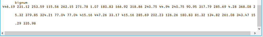
Fig. 3.1 A long variable being wrapped in the Windows IDE.#
Depending on the format in which you are reading this book, you may or may not be able to see all the numbers and they may or may not be laid out in several lines. If they are, then the first line will also not be indented, like in the figure above.
bignum ← 446.19 231.12 253.59 115.56 262.15 271.78 1.07 180.83 166.92 318.86 240.75 44.94 240.75 90.95 317.79 285.69 4.28 368.08 295.32 379.85 324.21 77.04 77.04 415.16 447.26 33.17 415.16 285.69 202.23 126.26 180.83 81.32 134.82 261.08 343.47 157.29 335.98
bignum
3.4. Simple Character Values#
3.4.1. Character Vectors and Scalars#
Up to now, we have used only numeric values, but we can also create textual data known as a character array. To identify a string of characters as text, we start and end it with a single quote:
text ← 'Today is August 7th, 2020'
text
⍴text
trailer ← 'I type 7 trailing blanks       '
trailer
⍴trailer
As these examples show:
the quotes are not part of the text, they’re just there to delimit it;
text can include any character: letters, digits and punctuation;
textandtrailerare vectors. They are sometimes called strings;APL does not recognize words; a character array is simply a set of characters; and
blank characters (spaces) are characters like any other character; they do not have any special meaning. However, when a character array is displayed any trailing blanks are most often invisible.
A problem may occur when the text itself includes an apostrophe, for example in a sentence like “It’s raining, isn’t it?”.
When you enter apostrophes as part of the text, you must double them, as shown below, to distinguish them from the delimiters:
damned ← 'It''s raining, isn''t it?'
This is only a typing convention, but the doubled quotes are transformed into a single apostrophe, as you can see here:
damned
As mentioned above, a character array can contain digits, but they are not considered to be numbers, and it is impossible to use them in a mathematical operation:
hundred ← '100'
hundred
hundred looks like a number, but it isn’t:
⍴hundred
hundred + 5
DOMAIN ERROR
      hundred+5
             ∧
Of course, a single character is a scalar:
singleton ← 'p'
⍴singleton
The result is a blank line because scalars have no dimensions.
≢⍴singleton
And the confirmation above tells us that singleton has 0 dimensions.
3.4.2. Character Arrays#
We saw, some pages ago, a list of months:
January
February
March
April
May
June
We can think of this as a list of 6 words, or as a matrix of 6 rows and 8 columns (the width of “February”). Both representations are valid, and both can be used in APL; let us study them one after the other.
To enter the months as a 6 by 8 matrix, one must use the reshape (⍴) function:
to the left of the function we must specify the shape of the matrix we want to build, which is
6 8; andto the right of the function we must specify all of the characters (including any trailing blanks) that are necessary to fill each row to the proper length.
Like so:
monMat ← 6 8 ⍴ 'January FebruaryMarch April May June'
No space was typed between February and March; do you see why?
Let us check the result:
monMat
Oops! We forgot that when the right argument is too short, ⍴ reuses it from the beginning. That’s the reason why the last row is wrong. We must add 4 trailing blanks.
Tip
You do not have to re-type the entire expression.
If you are working in the interpreter session, just move your cursor up to the line where you defined monMat, add the missing blanks, and press the Enter key.
APL will then copy the modified line down to the end of your session and automatically restore the original line to its original state. As a consequence, the interpreter window always displays the sequence of expressions and results in the order in which you typed them.
If you are working with the Jupyter notebook version of this book, you can just go to the input cell where you made your mistake and correct it in place. Otherwise, just copy the cell and correct the mistake in the copied cell:
monMat ← 6 8 ⍴ 'January FebruaryMarch   April   May     June    '
monMat
As expected, the shape of monMat shows it is a matrix:
⍴monMat
Now, to enter the months as 6 words, one must type each word between quotes, and check that each closing quote is separated from the next opening quote by at least one blank (otherwise it would be interpreted as an apostrophe - remember, the juxtaposition of two quotes in a character string is used to enter a single quote):
monVec ← 'January' 'February' 'March' 'April' 'May' 'June'
monVec
This, on the other hand, is a vector:
⍴monVec
monVec is a vector of a kind that we have not seen before, the items of which are 6 sub-arrays. This kind of an array is called a nested array and is the reason why we see those black boxes around the months.
Be patient! We shall study nested arrays very soon in this very chapter.
3.5. Indexing#
3.5.1. Traditional Vector Indexing#
Our variable contents contains the following items:
contents
To extract one of these items, you just have to specify its position, or index, between square brackets:
contents[3]
Of course, an index must follow some obvious rules: it must be an integer numeric value and it may not be negative or greater than the size of the vector, otherwise an INDEX ERROR will be reported.
It is possible to extract several items in a single operation, in any order, and you can even select the same item more than once:
contents[3 7 1 3 3 12]
The same notation allows you to modify one or more items of the vector. The only condition is that you must provide as many replacement values as the number of items you select, or give a single replacement value to use for all the selected items.
Below, we use three values to replace three items:
contents[2 4 6] ← 7 11 80
contents
Now we provide a single value to replace three items:
contents[8 11 12] ← 9999
contents
This works exactly the same on character vectors:
'COMPUTER'[8 7 4 2 8 6]
text ← 'BREAD'
text[2 4] ← 'LN'
text
3.5.2. The Shape of the Result#
The index may be a numeric array of any shape: scalar, vector, matrix, or an array of higher rank. To understand what happens, there is a simple rule.
Rule
When a vector is indexed by an array, the result has exactly the same shape as the index array, as if each item of the index had been replaced by the item it designates.
This rule is easy to verify. Let us restore the initial values of contents:
contents ← 12 56 78 74 85 96 30 22 44 66 82 27
And let us create a matrix of indices:
myIndex ← 3 5 ⍴ 5 5 4 4 8 6 12 6 11 12 10 6 1 4 9
myIndex
contents[myIndex]
For example, you can see that the index in row 2, column 5 was 12. So, it has been replaced by the 12th item of contents, i.e. 27.
The rule remains true if the indexed vector is a character vector. For example, imagine that we have a matrix named planning, in which some tasks are planned (1) or not (0) over the next 12 months:
⎕RL ← 73
planning ← ¯1+?5 12⍴2
planning
This is not very easy to interpret! Let us replace the inactive periods by “-“, and the busy periods by “⎕”. This beautiful character, named quad, can be entered by pressing APL+l.
'-⎕'[planning+1]
Isn’t it magic?
Do you understand why we added 1 to planning? Of course, the vector to be indexed was composed of only 2 characters, so the set of indices had to be composed only from the values 1 and 2 and that is why we used planning+1 to index.
All the 0’s in planning have been replaced by the 1st item (-), and all the 1’s have been replaced by the 2nd item (⎕).
3.5.3. Array Indexing#
Just to make some experiments, let us create a new variable, named tests:
⎕RL ← 73
tests ← ?6 3⍴100
tests
Indexing an array is very similar to the method we saw for vectors, but we now need one index for the row and one for the column; they must be separated by a semi-colon. For example, to get (or replace) the value 55 in row 4, column 3, one types:
tests[4;3]
It is of course possible to select more than one row and more than one column. If so, one obtains all the values situated at the intersections of the specified rows and columns.
tests[1 5 6;1 3]
The result of indexing may sometimes be surprising. Let us extract 4 values from the first column:
tests[1 2 5 6;1]
You probably expected the result to be displayed like a column? Really sorry!
The result of this expression is a vector, and a vector is always displayed as a row on the screen.
We shall see later that it is possible, using a little trick, to cause the result to be displayed vertically.
When you use indexing, you must specify as many indices or sets of indices as the array’s rank. For a 3D array, you must specify 3 sets of indices, separated by two semi-colons.
For example, suppose that we would like to extract the production of the 2nd assembly line, for the first 6 months of the last 2 years, from the array prod. Let’s express that in order of the 3 dimensions: Years/Lines/Months:
What we want |
Relevant indices |
|---|---|
The last 2 years |
4 5 |
The second assembly line |
2 |
The first 6 months |
1 2 3 4 5 6 |
prod[4 5;2;1 2 3 4 5 6]
The result above is a matrix: 2 (years) by 6 (months).
Remark
Because we can select rows and columns, the semi-colon is necessary to tell them apart.
For example, the indexing below gives rows 1 and 2, and column 3:
tests[1 2;3]
whereas
tests[1;2 3]
gives row 1, and columns 2 and 3.
Remark
It is also possible to select several items which are not at the intersections of the same rows or columns. To do so requires a special notation where the individual row/column indices of each item are embedded in parentheses. The reason for this syntax will become clear later, in the Section 3.6.
For example, let us select tests[2;3] together with tests[5;1] and tests[1;2].
tests[(2 3)(5 1)(1 2)]
3.5.4. Convention#
To specify all items of a dimension, you just omit the index for that dimension, but you must not omit the semi-colon attached to it.
In the previous example, to obtain both assembly lines we could have typed:
prod[4 5;1 2;1 2 3 4 5 6]
But it is shorter to type:
prod[4 5;;1 2 3 4 5 6]
The omitted index means “all the assembly lines”.
In the same way, omitting the last index means “all the months”:
prod[4 5;2;]
And finally, omitting the first and second indices means “all years and lines”:
prod[;;1 2 3]
This convention also applies to replacing specific items. For example, to change all the items in the last row of tests, we could type:
tests[6;] ← 60 70 80
tests
3.5.5. Warnings#
We would like to draw your attention to some delicate details now.
3.5.5.1. Shape Compatibility#
To replace several items in an array, the replacement array must have exactly the same shape as the array of indices they replace.
For example, suppose that we would like to replace the four “corners” of tests with the values 11, 22, 33, and 44, respectively.
We cannot successfully execute:
tests[1 6;1 3] ← 11 22 33 44
LENGTH ERROR
      tests[1 6;1 3]←11 22 33 44
           ∧
Notice the LENGTH ERROR that was issued (note that this is a “shape error”).
If we had extracted these four values, the result would have been a 2 by 2 matrix:
tests[1 6;1 3]
So, to replace them, we cannot use a vector, as we have just tried to do. Instead we must organise the replacement array into a 2 by 2 matrix, like this:
tests[1 6;1 3] ← 2 2 ⍴ 11 22 33 44
tests
Notice the corners have the new values.
3.5.5.2. Replace or Obtain All the Values#
To replace all of the values in an array with a single value, it is necessary to use brackets in which the indices of all the dimensions have been removed.
For example, imagine that we would like to reset all the values of tests to zero.
tests ← 0 would be wrong, because that would replace the matrix by a scalar.
The correct solution is
tests2 ← tests
tests2[;] ← 0
tests2
For a vector, like contents, we would write
contents[] ← 123
contents
to replace all the items with 123.
3.5.5.3. “Pass-Through” Value#
Imagine that we have a vector:
vec ← 32 51 28 19 72 31
We replace some items and assign the result to another variable:
res ← vec[2 4 6] ← 50
What do we get in res? Is it res ← vec[2 4 6], or is it res ← 50?
res
In fact, we get 50. We say that 50 is a pass-through value.
3.5.6. The Index Function#
In APL, nearly all of the built-in functions (known as primitive functions) are represented by a single symbol: + × ⍴ ÷ etc. Bracket indexing, as we introduced above, is an exception: it is represented by two non-contiguous symbols, [ and ]. This is one of the reasons why modern versions of APL also include an index function.
It is represented by the symbol ⌷. Beware: this is not the symbol quad used in our planning example a few pages ago! In fact, it looks like a quad which has been squished, hence its name: squish-quad, or squad for short. The squad is obtained with APL+Shift+L. When applied to a vector, index takes a single number on its left:
3 ⌷ contents
The above is equivalent to contents[3].
For now, we shall not try to extract more than one item from a vector; we need additional knowledge to do that.
For a matrix, index takes a pair of values (row/column) on its left.
4 2 ⌷ tests
The above is equivalent to tests[4;2].
It is possible to select several rows and several columns, using a special notation that will be explained in subsequent sections. The left argument of Index is now made of a list of rows followed by a list of columns, both parenthesised:
(1 3 6)(1 3)⌷tests
This is equivalent to tests[1 3 6;1 3].
3.5.7. Even More Indexing#
APL provides other syntaxes and functions that allow you to index into arrays. They will be introduced later in Section 10.2, Section 10.11, and Section 10.10. You do not need to rush to those sections to learn about this right now, this is only to let you know that you will learn more techniques when the time comes.
3.6. Mixed and Nested Arrays#
Up to now we have dealt only with homogeneous arrays: scalars, vectors or higher rank arrays containing only numbers or only characters. An array was a collection of what we call simple scalars. In the early 1980’s enhanced versions of APL started to appear. They accepted a mixture of numbers and characters within the same array (so-called mixed arrays), and arrays could contain sub-arrays as items (so-called nested arrays).
In this chapter, we shall explore only some basic properties of mixed and nested arrays, just to help you understand what might otherwise appear to be unusual behaviour or unexpected error messages. We shall not go any further for now; the “Nested Arrays (continued)” chapter will be entirely dedicated to an extensive study of nested arrays.
Note that with the current widespread use of nested arrays, it is now very common to refer to an “old-fashioned” array that is not nested as a simple array.
3.6.1. Mixed Arrays#
An array is described as a mixed array if it contains a mixture of scalar numbers and scalar characters.
It is easy to create such an array:
mixVec ← 44 87 'K' 12 29 'B' 'a' 'g' 46.3
⍴mixVec
This mixVec is a vector. Check how it looks like:
mixVec
mixMat ← 2 5⍴mixVec
⍴mixMat
mixMat is a matrix and looks like
mixMat
3.6.2. Four Important Remarks#
In a vector like
mixVec, each letter must be entered as a scalar: embedded within quotes, and separated from the next one by at least one blank space.
If the space is omitted, for example, if we type
'B''a''g'
APL interprets the doubled quotes as apostrophes, which yields B'a'g. This is not a sequence of 3 scalars, but a 5-item vector:
≢ 'B''a''g'
If we insert the proper spacing, we get a vector with 3 items:
≢ 'B' 'a' 'g'
When
mixVecis displayed (see above), the three lettersBagare joined together, like the letters in any vector of characters.
This presentation might be confused with an array of 7 items, whose 6th item is the vector 'Bag'. That would be a nested array. We will soon learn how to investigate the structure of an array.
This confusion disappears in
mixMat. Because the items of the matrix must be aligned in columns, “B” is placed under 44, “a” under 87, and “g” under “K”. Here you can easily see that the three lettersBagare really three independent scalars.A mixed array is made up only of simple scalars (numbers or characters); it is not a nested array.
3.6.3. Nested Arrays#
An array is said to be generalised or nested when one or more of its items are not simple scalars, but are scalars which contain other arrays. The latter may be simple arrays of any shape or rank (vectors, matrices, arrays), or they may themselves be nested arrays.
A nested array can be created in a number of ways; we shall begin with the simplest one, known as vector notation, or strand notation. In strand notation, the items of an array are just juxtaposed side by side, and each can be identified as an item because it is:
either separated from its neighbours by blanks;
embedded within quotes;
an expression embedded within parentheses; or
a variable name.
Just to demonstrate how it works, let us create a nested vector and a nested matrix.
We start with two simple arrays:
one ← 2 2 ⍴ 8 6 2 4
two ← 'Hello'
Which will now be used to create more involved arrays:
nesVec ← 87 24 'John' 51 (78 45 23) 95 one 69
≢nesVec
The length of nesVec is 8 because we have juxtaposed 8 items.
nesVec
The Jupyter notebook puts boxes around the items of the vector to make it easier to interpret the result. If the expression above were to be run in the Dyalog APL interpreter session, the result would be
87 24  John  51  78 45 23  95  8 6  69
                               2 4
which is a bit difficult to read and interpret.
And now, a matrix!
nesMat ← 2 3 ⍴ 'Dyalog' 44 two 27 one (2 3⍴1 2 0 0 0 5)
⍴nesMat
nesMat
Again, the notebook boxes the items of the matrix so we have an easier time interpreting the result. In the interpreter session the output would be
 Dyalog   44  Hello
     27  8 6  1 2 0
         2 4  0 0 5
To obtain this kind of boxed presentation in the interpreter session, execute the following command (remember that a command begins by a closing parenthesis):
)copy Util DISP
Then execute:
DISP nesMat
If you want this kind of boxing to be permanent, you can go to your session and type
]box ON
which, on your interpreter session, should actually print Was OFF, meaning that automatic boxing of nested arrays was OFF and now is ON. Because Jupyter notebooks have this option ON by default, typing ]box ON tells the option was already ON.
For demonstration purposes, we will turn the automatic boxing OFF to compare the results of viewing nesMat without having to use the DISP function:
nesMat
]box OFF
nesMat
DISP nesMat
You probably remember the mixed vector mixVec, which contained three adjacent scalars, “B”, “a”, and “g”. Let us compare the unboxed display of mixVec with a seven item nested vector, whose sixth item contains the word “Bag”:
44 87 'K' 12 29 'Bag' 46.3
Now we look at mixVec:
mixVec
If you look closely you will have observed that, in the nested array, the sub-vector Bag is separated from its neighbours not by a single space, but by two spaces: this should alert an experienced APLer that it is a nested array. However, this difference is so small that the APL community, all over the world, uses a utility program, named DISPLAY, to draw boxes around arrays (nested or not) to make things clear. Let us examine it in the next section.
Notice that because mixVec is not nested it has no boxes around its items.
3.6.4. DISPLAY#
DISPLAY is provided with Dyalog APL in a library workspace which itself is named DISPLAY. Because this library is by default on the Workspace Search Path of APL, you can easily add the DISPLAY function to your active workspace by typing the command:
)copy DISPLAY
This command copies the entire DISPLAY workspace into your current session, but it contains only one single function: DISPLAY.
As you can see, applied to a simple scalar, DISPLAY already produces slight differences:
37
DISPLAY 37
'K'
DISPLAY 'K'
We see that the display results are centered in a three row area; for numerical simple scalars the top and bottom rows are empty, which creates the white region around the 37 you can see above. For character simple scalars, the bottom row underlines the character and the top row is left empty.
However, applied to a vector, DISPLAY will provide more information:
DISPLAY 54 73 19
In the example above we can see that the default presentation uses line-drawing characters to draw the box. This means in the Windows IDE, in RIDE, and in the Jupyter notebooks you should see a continuous frame around the vector. However, if you are reading this book online the framing might look “broken”.
The second, rougher, form of presentation is provided for use in circumstances where the line-drawing symbols in the APL font are not displayed or printed as intended. This will depend upon your version of the Operating System and on the display and printer drivers you are using.
3.6.4.1. Conventions#
The upper-left corner of the box provides information about the shape of the displayed value:
a single horizontal arrow for a vector;
two (or more) arrows for a matrix or higher rank arrays; and
no arrow at all for scalars containing nested values (a concept we haven’t seen up to now).
The bottom-left corner of the box provides information about the contents of the array:
~means that the array contains only numeric values;-(which actually goes unnoticed) means that the array contains only characters;+is used for mixed arrays; and∊means that the array contains other arrays: it is a nested array.
3.6.4.2. Examples#
numeric (
~) vector (→):
DISPLAY 78 45 12
matrix (
→→); because of its two arrows, this matrix cannot be confused with the vector shown above.
DISPLAY 1 3 ⍴ 78 45 12
character (
-) matrix (→→); because of the line-drawing characters, the bottom-left corner of this matrix looks like it doesn’t even have information on the type of the values the matrix contains.
DISPLAY 2 6 ⍴ 'Sunny Summer'
numeric (
~) array with three dimensions (→→→):
DISPLAY prod[1 2;;1 3 5]
Mixed arrays are sometimes more complex to understand. For example, here is a
mixed (
+) vector (→):
DISPLAY 54 'G' 61 'U' 7 19
Here is another vector with the same DISPLAY structure, but where the type of each item is harder to identify:
DISPLAY 54 3 'G' 'U' 7 '3' 19
Note that in the example above it is impossible to distinguish between the numeric value 3 and the character value '3'. The DISPLAY function actually tries to help us by underlining all character values, but unfortunately this coincides with the bottom border of the box. When the array being displayed becomes more complex, you will see this underlining, as the next example shows.
The two adjacent scalars 'G' and 'U' are displayed side by side; a vector 'GU' would have given a nested array, with a different representation, as you can see below:
DISPLAY 54 3 'GU' 7 '3' 19
Notice that, because one of the items of this array contains a vector, the array is nested, hence the ∊ sign at the bottom-left corner. Now the underlining of '3' is visible, so it is easy to see that it is a character. Since 7 is not underlined it is a number.
We shall discover more about DISPLAY in Section 10.1.3 when we study nested arrays in detail, but we can already use it to show the structure of the arrays that we have been working with. For example, our nested matrix nesMat:
DISPLAY nesMat
You can see that all the sub-arrays contained in nesMat are individually represented with the same conventions, making the interpretation easy.
3.6.5. Be Simple!#
Up to now, the nested arrays we have met contained only “simple” items (scalars, vectors, matrices). Here is a completely weird matrix, which itself contains a small nested array made of the first two columns of nesMat:
weird ← 2 2 ⍴ 456 (nesMat[;1 2]) (17 51) 'Twisted'
weird
Notice how the default presentation makes it difficult to interpret the contents of weird. We can use DISPLAY to make things clearer:
DISPLAY weird
Remark
Of course, even if APL can handle arrays as unusual as the one above, it is not advisable to build such arrays! Most nested arrays have a clear and straightforward structure.
Remember that earlier we had a list of month names to store, and we had the choice between storing them in a matrix or in a vector of vectors (that is to say, a nested vector).
monVec
Because its contents are homogeneous (made up only of vectors), this array has a simple structure that is clear and easy to interpret. DISPLAY shows it like this:
DISPLAY monVec
Imagine now that we want to store the ages of the children of five families; we could enter them like this:
children ← (6 2) (35 33 26 21) (7 7) 3 (19 14)
children
DISPLAY children
This array is not homogeneous; it is made of vectors mixed with a scalar. However, its structure is simple, and consistent. Together with the previous example, it is a pertinent usage of nested arrays.
3.6.6. That’s Not All, Folks!#
In this section we have only described some basic things about nested arrays. APL provides a number of functions designed specifically to manipulate nested arrays, but it would be premature to introduce these now until we have fully explored all of the basic capabilities. Nevertheless, if you want to learn a bit more on the subject, just skip to the chapter on nested arrays.
3.7. Empty Arrays#
An array is an empty array if the length of one or more of its dimensions is zero. Hence, it is possible to meet many different kinds of empty arrays: vectors, matrices, arrays of any rank or type.
Here are some examples:
empty numeric vector:
0⍴0
empty numeric vector (because nothing was typed between the quotes):
''
However, the following is not an empty vector, given that we typed a blank character. Though invisible, it is a character just like 'B' or 'z':
' '
empty character matrix with 0 rows and 3 columns:
0 3⍴''
empty numeric matrix with 5 rows and 0 columns:
5 0⍴0
Notice how the empty vector with 5 rows (but 0 columns) took up more vertical space than the empty vector with 0 rows (and 3 columns).
empty numeric array of rank 3:
3 0 7⍴0
There are many ways to create empty arrays, as we shall discover in the following chapters.
We shall see later that empty arrays, which you may find surprising, are extremely useful in solving a large number of business problems. In fact, they are often used as the starting point (initial value) for variables that will grow by the iterative addition of new items.
The empty numeric vector is probably the most frequently used of all empty arrays. For that reason, a special symbol has been designed to represent it: ⍬ (entered by pressing APL+Shift+]).
Because this symbol is made of a zero with a tilde on top of it, it is called zilde.
Let us conclude this topic with a rather comforting statement. We start with an empty vector:
emptiness ← ⍬
Now we create a text vector:
presence ← 'Friendly'
We then give presence the shape of emptiness…
emptiness ⍴ presence
And it works!
This proves that a friendly presence can fill up emptiness! That’s good! But can we explain it? Let’s try…
In the last expression, the reshape function (⍴) returns an array with the shape specified in its left argument emptiness.
Since emptiness is an empty vector (⍬), reshape will return an array having an empty shape. Such an array is a scalar, so we know that the result of the expression will be a scalar.
Reshape will also fill the scalar with a value, taken from the right argument presence. presence contains the character vector 'Friendly', but since we only need one item to fill a scalar, we can only use the 'F'. The rest of the character vector 'Friendly' is not used.
In fact, the expression ⍬⍴array is widely used to return the first item of an array as a scalar, and in particular to convert a 1-item vector into a scalar.
Remark
Though they both are invisible when displayed, a numeric empty vector (⍬) is different from a character empty vector ('').
3.8. Workspaces and Commands#
You have nearly finished this chapter and, naturally, you would like to save the variables you have created. If you are using the Windows IDE you have two graphical ways of doing so:
in the “File” menu, select “Save” or “Save as”, and use the normal procedure for saving a file (highlighted in red below); or
you can click, in the toolbar, on the icon of a diskette (also highlighted in red below; who still knows what a diskette is?), which is equivalent, in APL, to “Save as”.
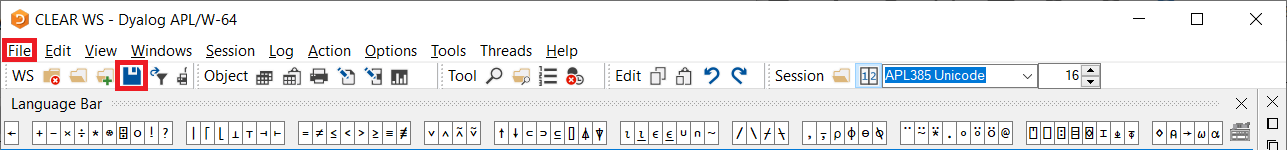
Fig. 3.2 Windows IDE toolbar with the “Save” toolbar shortcut and the “File” menu highlighted.#
If you are using RIDE or if you don’t like clicking menu buttons,
there is also a built-in method in APL, which may be activated through a special save command or function, as will be described later in this Section.
An explanation of how APL manages your data in the interpreter session is given below.
3.8.1. The Active Workspace#
When you start a working session with APL, you are allotted an empty portion of memory, which is called a workspace, or WS for short. This WS is called the active WS, because it is the area of memory in which you work. You gradually fill it with variables and functions2 as you create them.
² In APL we try to design a computer program, not as a single monolithic procedure, but rather as a set of inter-connecting units known as functions (or user-defined functions to distinguish them from primitive or built-in functions). Each function is ideally small, self-contained, and performs a single specific task.
You can ask the system to give you the list of your variables and functions. To do that, you use a system command: a special word which is recognised by the APL system because its first character is a closing parenthesis: ). Some Swedish APLers call that a “banana”.
The names of system commands are not case sensitive; they can be typed in mixture of upper and lower-case characters.
Let’s obtain a list of our variable names, using the command )vars:
)vars
The variables are listed in alphabetic order, but beware, the lower-case alphabet is ordered after the upper-case one.
If some of these variables are no longer useful, we can delete them with the following command, in which the variable (and function) names can be listed in any order:
)erase tests contents nesmat
We misspelled the name of one of our variables; the system erased the other ones, and gave us a warning. We can re-issue a command to erase the variable nesMat:
)erase nesMat
This example underlines the fact that although the command name (“erase”) itself is not case sensitive, the names that it is instructed to work on are of course still case sensitive.
If you had developed functions, you could list them using the command )fns (pronounced “funs”):
)fns
Because we developed no functions we only see the functions we loaded earlier on.
Remark
One can erase everything from the active workspace (all variables and all functions etc.) and revert to the original “clear” active workspace, by issuing the command )clear.
)clear
Now all variables are gone:
)vars
and so are all the functions:
)fns
This is a bit brutal: all of the contents of the WS are deleted, and no warning message is issued to notify the user of the consequence before the execution of the command. You should avoid using this command, and instead use the “Clear” button on the interpreter toolbar (highlighted in red below), which asks for confirmation. It is safer.
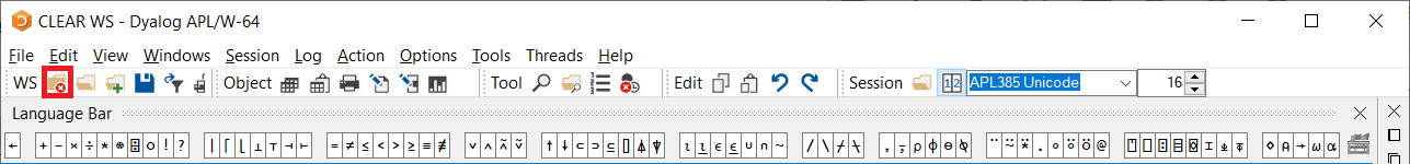
Fig. 3.3 Windows IDE with the “Clear” toolbar shortcut highlighted.#
Remark
In many languages, programs must be stored (saved) independently, one after the other, and variables do not exist on their own: they live only during the execution of a program which creates, uses and destroys them.
In APL, things are different:
variables can have an independent existence, outside of any program execution; you have seen that it is possible to create variables and manipulate them, at will, without writing any programs. This is similar to the interpreter sessions of some other languages, like Python or MATLAB; and
there may be a permanent interaction between programs and variables. Saving only any part of them would be nonsense: one must save the whole context; in other words, one must save the whole active workspace.
This is what we shall discover now.
3.8.2. The Libraries#
Like in most other software environments:
when you save a WS for the first time, you must give it a name; and
once it has been saved you need not re-specify its name when you re-save it.
Furthermore, we advise you to not re-specify the name when you want to re-save your work, because, if you misspell it, your WS will be saved with the wrong name without you being aware of it.
To save a WS, just issue the command )save followed, if this is the first time, by a file name. Let us create a simple variable and recreate the prod variable and then save them in an example workspace:
text ← 'The quick brown fox jumps over the lazy dog.'
⎕RL ← 73
prod ← ?5 2 12⍴50
)save MyPreciousWS
A confirmation message appears, specifying where it has been saved, and the date and time of the operation.
Of course, you can specify any path in your command, to save your WS wherever you like, but if you want to specify a full path, it is often more convenient to use the “Save” button in the toolbar, and browse through your folders.
You can have dozens of workspaces saved in various folders, according to your needs; they represent your private library.
You can also use public workspaces provided by Dyalog Ltd. as part of the APL system, workspaces downloaded from web sites, or workspaces provided by third-party developers.
You can list your workspaces using the command )lib.
Used alone, the command explores only the folders specified in your configuration parameters, which can be modified using the interpreter menu: “Options” ⇨ “Configure…” ⇨ “Workspace” ⇨ “Workspace search path”.
You can also specify explicitly in which folder the command should search:
)lib .
Only one workspace was found in the same folder as this notebook.
3.8.3. Load a WS#
Once a WS has been saved, it may be used again in various ways:
you can double-click on the WS name in your operating system’s file explorer;
you can use the menu “File” ⇨ “Open”;
you can click on the “Open” icon in the toolbar (highlighted in red below); or
you can issue the system command
)load
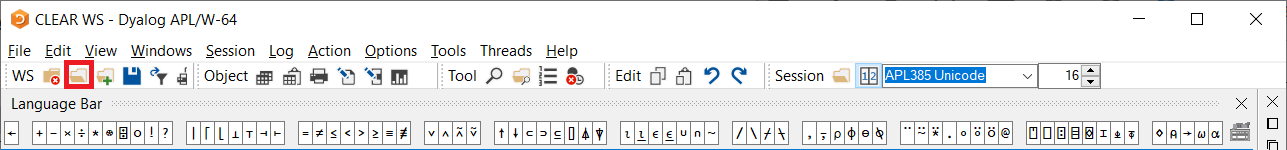
Fig. 3.4 Windows IDE with the “Load” toolbar shortcut highlighted.#
In all these cases, you will see the familiar file search box, in which you can browse to and select the workspace file you would like to open (or load).
You can also use the )load command followed by a WS name:
)load MyPreciousWS
In this case APL will search for your workspace in the folders specified in your workspace search path as explained above, unless you specify a full path name. If the path name includes blank characters, you must place the whole expression between double quotes, as in the first example below:
      )load "d:/my documents/sixteen tons/coal" ⍝ double quotes are mandatory.
      )load e:/freezer/mummies/ramses2          ⍝ double quotes are not needed.
Remark
When a WS is loaded, it replaces the active WS in memory and becomes the new active WS. If you have not saved the variables and functions you were working on, they are definitely lost! There is no warning message.
You must be aware of this because in this respect, APL differs from most software environments, in which each new file you open is opened in a separate window.
Remark
When a WS is loaded, a confirmation message appears, like the following:
.\MyPreciousWS.dws saved Sat Oct 3 19:31:42 2020
Note that the date and time reported is the date and time when the WS was last saved.
3.8.4. File Extensions#
The default extension of an APL WS depends on the APL system you use. For Dyalog APL, the extension is dws, an acronym for Dyalog WorkSpace.
This is only a default extension. When you save a WS, you can give it a different extension, like “old”, “std” or “dev”.
If you do so, you must be aware that when you load a WS using the )load command, and omit the extension, the command will only search for files with a dws extension.
Imagine that you have saved a WS under the name weekly.old. This WS will not be found if you just issue the command )load weekly. You must specify the extension: )load weekly.old.
All these considerations are not mandatory knowledge, since you can navigate through the file search dialog box, or through your operating system’s file explorer.
3.8.5. Merge Workspaces#
Suppose that you would like to use some functions or variables stored in another WS that has previously been saved. You can import them into your active WS using the command )copy, followed by the name of the WS and then the names of the functions and variables you want to import.
For example, imagine that you need Screwdriver, Hammer and Saw, all stored in a WS named Toolbox. You can issue the command
)copy Toolbox Screwdriver Hammer Saw
The WS name must be the first (under Microsoft Windows it is not case sensitive) and the names of the functions and variables must follow, but beware, these are always case sensitive.
If you specify only the workspace name, all its contents are imported. Be sure that all that stuff is really useful to you.
When the copy is complete, a confirmation message is issued. Like the message issued by a )load command, it tells you when the WS was last saved.
Of course, you can specify a path in the command; otherwise the WS is searched for in the workspace search path defined in your configuration. Once again, use double quotes if necessary:
)copy "d:/my documents/recipes/ratatouille"
3.8.5.1. Protected Copy#
When you import the entire contents of another WS, there is a risk that it contains an object (variable or function) which has the same name, but not the same value, as an existing object in your active WS. If so, the imported object replaces the current one. Danger!
You can avoid this by using the )pcopy command, with the P standing for “Protected”. If there is a name conflict, the object in the active WS is not overwritten, and a message tells you which objects haven’t been copied. Let’s demonstrate this. First we clear our current WS to simulate a fresh start:
)clear
Now we define some variables that are useful for our calculations:
text ← 'This is just some text.'
≢text
And now we import the contents of the auxiliary WS because we need it as well:
)pcopy MyPreciousWS
Notice how text was not copied from the auxiliary WS because we have defined our own text above.
3.8.5.2. Intentionally Destructive Copy#
We saw that an imported object may overwrite an object in the active WS. This is sometimes useful!
Imagine that you loaded the WS:
)load MyPreciousWS
Then you spend some hours adding new functions and variables, changing things here and there, and suddenly, you discover that you made inappropriate changes to text.
You can retrieve the original variable, still present in the saved version of MyPreciousWS, with:
)copy MyPreciousWS text
When imported, the original version of text will override the version you mistakenly altered. Your active workspace will be correct again, and you will be able to go on with your work (but don’t forget to save it!).
Of course this becomes more helpful if you have many more variables in your workspace. If you had made some useful changes to text you wouldn’t want to copy the whole workspace into your active workspace, hence the usefulness of the command demonstrated above.
3.8.5.3. Evolution of Your Code#
Imagine that you have imported into your active WS a function named Compute, copied from a WS named Utilities. When you save your active WS, for example under the name Budget, the function Compute will be saved with it.
But now, imagine that the original version of the function Compute contained in Utilities is modified, or enhanced; what happens? The copy saved with Budget is still the old version, and Budget may therefore be outdated.
This is a reason why APL allows a dynamic copy of what you need from a known reference WS. This technique will be explained in the chapter on system interfaces.
3.8.5.4. Active WS Identification#
You can obtain the name of your current WS by issuing the command:
)wsid
Do not be misled by the name that is reported: it just means that the contents of your active WS had initially been loaded from that WS, or have recently been saved under that name. But since it was loaded or saved, your current WS may have been modified, and may no longer be identical to the original copy stored in the library.
In the same way, if you see instead the message "is CLEAR WS", it does not mean that your WS is clear (empty; contains nothing), but that is has not been saved yet, and hence has no name.
3.8.6. Exiting APL#
You can close an APL session using three traditional Windows methods, and two APL system commands:
you can click on the “Close” cross at the top-right corner of your APL window;
you can press Alt+F4;
you can activate the menu “File” ⇨ “Exit”;
you can issue the system command
)off; oryou can issue the system command
)continue.
The first two methods will ask if you want to save your current session configuration, a so called “continue WS” (this will be seen in a later chapter), and the log of everything that you did during the session. The next two methods will close APL without any question or warning, and will not save your configuration. The last one will save a continue WS before exiting.
In any case, always remember to save your work (if necessary) before you quit.
3.8.7. Contents of a WS#
Generally speaking, a workspace contains functions and variables which interact to constitute some useful application.
The large memories of modern computers support very big workspaces, and a single WS is generally enough to store even a very complex application, or several applications. However, it is good practice to store different applications in different workspaces: accounting, budget, customer care, etc. It is not recommended that you mix several applications in a single WS.
However, if appropriate, it is possible for a function to dynamically load another workspace (without any intervention by the user), and activate a different or complementary application.
For now, a unique WS should be sufficient to contain all your experiments.
If several workspaces need to share a command set of utility programs, this can be accomplished by dynamically importing the utilities from a common source. This will also be seen in the chapter on system interfaces.
3.8.8. Our First System Commands#
Just to recapitulate, here is a little summary of the system commands we’ve just discovered. Many other commands will be studied (cf. the chapter on system interfaces). The following conventions are used in the table below:
the command names are writing using normal characters; the parameters are in italics;
parameters within {braces} are optional;
names represents a list of variable or function names; and
wsname is the name of a WS:
this name may contain a file extension, which is only necessary if it is different from “dws”; and
this name may also be preceded by an optional path. If the path is not specified, APL searches in some default directories. (In the Windows IDE, you can change those directories under “Options” ⇨ “Configure…” ⇨ “Workspace” ⇨ “Workspace search path”.)
Command |
Usage |
|---|---|
|
Lists the variables in the active workspace. |
|
Lists the user-defined functions in the active workspace. |
|
Deletes the named objects from the active workspace. |
|
Deletes everything and leaves the active workspace empty. |
|
Saves the active workspace under its current name, or: opens the File Save dialog box if the WS has no name yet. |
|
Saves the active WS under the given path/name/extension. |
|
Gives the list of all workspaces in the workspace search path. |
|
Gives the list of all workspaces in the specified path. |
|
Deletes a saved WS from disk. |
|
Opens the File Open dialog box, from which a workspace can be selected. It will replace the active WS. |
|
Replaces the contents of the active WS with the referenced WS. |
|
Imports the named items from the specified WS into the active WS, where they may overwrite objects identically named. |
|
Imports all contents of the specified WS. |
|
Similar to |
|
Displays the name of the current (active) WS. |
|
Closes the APL session. |
|
Saves a continue WS and closes the APL session. |
3.9. Exercises#
Warning
The following exercises are designed to train you, not the computer.
For this reason, we suggest that you try to answer them on a sheet of paper, not on your computer. When you are sure of your answer, you can test it on the computer.
Exercise 3.1
Given a scalar s, can you transform it into a vector containing one single item? What about the opposite: can you transform a one-item vector v into a scalar?
Exercise 3.2
Define x so that this interactive session becomes possible:
      x
2 15 8 3
      ⍴x
8
Exercise 3.3
Find the result of this expression: 'LE CHAT'[7 5 2 3 4 6 7]. This amusing example was first given in “Informatique par telephone” of Philip S. Abrams and Gérard Lacourly, Editions Herman, Paris 1972.
Exercise 3.4
The variable tab is created like this:
tab ← 2 5 ⍴ 9 1 4 3 6 7 4 3 8 2
How could you replace the values 9 6 7 2 in this variable by 21 45 78 11 respectively?
Exercise 3.5
Consider the following assignments:
x ← 1 2 9 11 3 7 8
x[3 5] ← x[4 1]
What do you think is the new value of x? And what happens if you now execute
x[4 6] ← x[6 4]
Exercise 3.6
A vector of six items named mystery is indexed like this:
      mystery[3 1 6 5 2 4]
8 11 3 9 2 15
What is the value of mystery?
Exercise 3.7
One creates a vector, and selects some items from it, as shown:
      vec ← 33 19 27 11 74 47 10 50 66 14
      vec[findMe]
47 27 19 14 50 74
Could you guess the value of findMe?
Exercise 3.8
One creates a vector, and a set of indices:
source ← 10 4 13 3 9 0 7 6 2 13 8 1 5
set ← 3 3 ⍴ source[2 4 8 5 12 13 7 4]
Then one uses it to index the original vector:
result ← source[set]
What is the shape of result? Can you find its value?
Exercise 3.9
Is there a difference between the following two vectors?
v1 ← 'p' 'o' 't'
v2 ← 'pot'
Exercise 3.10
Is there a difference between the following two vectors?
v3 ← 15 48 'Y' 'e' 's' 52
v4 ← 15 48 'Yes' 52
Exercise 3.11
Here is a very simple variable:
two ← 2
We use it in the following expression:
foolish ← two two ⍴ 2 two '⍴' 'two'
What is the shape of foolish? Can you find its value?
Proposed solutions to the exercises can be found in Section 3.11.
3.10. The Specialist’s Section#
You will find here rare or complex usages of the concepts presented in this chapter, or discover extended explanations which need the knowledge of some symbols that will be seen much further in the book.
If you are exploring APL for the first time, skip this section and go to the next chapter.
3.10.1. Variable Names#
Variable names must obey the rules shown in Section 3.1.2.
We have seen that you may use some special characters: delta (∆), underscore (_), and also the underscored delta (⍙). We do not recommend these symbols; they often make programs difficult to read.
3.10.2. Representation of Numbers#
Up to now, we have entered decimal numbers using the most common conventions, like 3714.12 or 0.41.
It is also possible to employ other conventions to facilitate typing.
When the magnitude of a decimal value is less than 1 it is not necessary to enter a zero before the decimal point:
.413
¯.5119
Very large and very small numbers can be entered using scientific (or exponential) notation.
Using this convention, any “extreme” number can be represented by a “normal” number, the mantissa, multiplied by a power of 10, the exponent.
For example, 42781900 could be represented as:
and 0.0000038421 could be represented as:
In APL, the mantissa and the exponent are separated by the letter E.
Using this notation, one can enter very large or very small numbers with ease. Beware that, strictly speaking, scientific notation requires the mantissa to be a number between greater than or equal to 1 and lower than 10, but this notation works in APL even if the mantissa doesn’t fall within that range.
If the magnitude of the number is not too large nor too small, all its digits will be displayed:
4.27819E7
4278.19E4
384.21E¯8
3.8421E¯6
But if the numbers are very large (or very small), and would require more digits to be shown than the maximum (defined by ⎕PP, the print precision) APL displays them with a “normalised” mantissa with only one non-zero digit, followed by some decimal places (if any) and the appropriate exponent:
431765805838751234
5678.1234E20
1234.9876E¯15
¯2468.1357E¯13
3.10.3. The Shape of the Result of Indexing#
Rule
Suppose you are given an array of any rank array.
The expression array[a; b; c; ...] always gives a result with a shape equal to (⍴a),(⍴b),(⍴c),....
This rule makes it possible to always predict the shape of the result of an indexing operation.
For example,
prod[2 5 3;2 1;1 2 5 6]
gives a result of shape 3 2 4. Similarly,
prod[;2;⍳6]
gives a result of shape 5 6.
In the last example, the omitted index refers to the first dimension of prod which is of length 5.
The second index (2) is a scalar, and has no dimension.
That’s why the shape of the result is 5 6 and not 5 1 6.
3.10.3.1. Using Ravel to Preserve a Dimension#
Usually, a matrix is indexed like mat[rows;cols], for example
mat ← prod[;1;]
rows ← 1 2
cols ← 3 6
mini ← mat[rows;cols]
mini
Generally, rows may contain several row numbers, and cols may contain several column numbers. Applying the preceding rule, it is easy to see that we’ll obtain a sub-matrix mini.
But it may be that rows or cols are scalars. The result of mat[rows;cols] would then not be a sub-matrix, but a scalar or a vector. This could lead to other expressions in your function generating an error or an incorrect result, because they were written expecting matrices.
rows ← 1
mini ← mat[rows;cols]
mini
⍴mini
By checking the shape of mini, we can see mini is a vector now.
If cols is also a scalar, then mini becomes a scalar:
cols ← 6
mini ← mat[rows;cols]
mini
⍴mini
To avoid this problem, you can force an index expression to be a vector (perhaps a vector containing only one item) by using ravel (,) like this:
mini ← mat[,rows;,cols]
mini
⍴mini
Now mini is the correct 1 by 1 matrix we wanted it to be.
Ravel shall be discussed in Section 4.16.
In Section 3.5.3, we indexed a matrix in a way similar to this:
mat[1 2 5;1]
And we were surprised to see the values of a column were displayed horizontally. We can now understand why: the shape of the result is equal to (⍴1 2 5),(⍴1). As the shape of a scalar is empty, this expression is equivalent to (⍴1 2 5), i.e. 3. The indexing operation therefore produces a vector, which is displayed on a single line of the screen.
To obtain a matrix, we must transform the column index (scalar 1) into a vector: we shall again use ravel, like this:
mat[1 2 5; ,1]
3.10.4. Multiple Usage of an Index#
When an array is indexed, the same item (the second item in the example below) may be selected more than once; for example:
a ← 71 72 73 74 75 76
a[2 3 2 4 2]
If a repeated index is used to update the variable, only the last replacement value is retained:
a[2 3 2 4 2] ← 45 19 67 33 50
a
In the assignment above, the second item was set to 45, then 67 and finally 50.
3.10.5. A Problem With Using Reshape (⍴)#
We want to create a numeric matrix with 3 rows, and as many columns as another matrix mat, entirely filled with zeros.
One solution is to first obtain the number of columns of mat, using the drop (↓) function (to be discussed later):
1↓⍴mat
We can see mat has 12 columns. Now we can manually build the correct matrix using the number of columns (12) we obtained previously:
3 12⍴0
Now let us try to build a generalised solution:
nc ← 1↓⍴mat
new ← 3 nc⍴0
DOMAIN ERROR
      new←3 nc⍴0
              ∧
But it no longer works!
The reasons for the problem are as follows:
when, in the first example, we entered the expression
3 12, we juxtaposed two scalars, and the result was a two-item vector;the expression
⍴matin the second example returns a two-item vector (5 12to be more precise). The function drop leaves only one value, but the result12is still a one-item vector; andwhen we then entered the expression
3 nc, we juxtaposed a scalar to a vector. This does not return a simple vector, but a nested array.
Unfortunately, a nested array is not a valid left argument for reshape! To solve this, we catenate 3 and nc to form a simple vector, which we then use as the left argument to ⍴ (catenate is also discussed later on).
new ← (3,nc)⍴0
new
A direct solution would be:
new ← (3,1↓⍴mat)⍴0
new
3.10.6. Monadic Index, or Materialise (⌷)#
In Section 3.5.3, we used the index function with a left argument for indexing.
Used monadically (without a left argument), materialise returns all the items of its right argument, whatever its shape:
vec ← 17 41 23 64
⌷ vec
mat ← 2 3 ⍴ ⍳6
⌷mat
The materialise function may also be used with Objects (See Chapter Q, Object Oriented Programming). Applied to an enumerate property of an object, or an instance of an object which has such a property as its default property, the same syntax returns all the items in this collection.
For example, to obtain the names of all the sheets in an Excel workbook, one can type:
XL.ActiveWorkbook.(⌷Sheets).Name
In this expression, ⌷Sheets represents the collection of all those sheets.
3.11. Solutions#
The following solutions we propose are not necessarily the “best” ones; perhaps you will find other solutions that we have never considered. APL is a very rich language, and due to the general nature of its primitive functions and operators there are always plenty of different ways to express different solutions to a given problem. Which one is “the best” depends on many things, for example the level of experience of the programmer, the importance of system performance, the required behaviour in border cases, the requirement to meet certain programming standards and also personal preferences. This is one of the reasons why APL is so pleasant to teach and to learn!
We advise you to try and solve the exercises before reading the solutions!
Solution to Exercise 3.1
The dyadic use of ⍴ is reshape, so that is what we are going to do to turn a scalar
s ← 2
into a 1-element vector. A 1-element vector has shape 1, so
1⍴s
will do the trick, even though it may look like it didn’t work. If we check the ranks, we can see it did; a scalar has rank 0,
≢⍴s
whereas a vector has rank 1:
≢⍴ 1⍴s
To go the other way around we just have to remember that a scalar has an empty shape, that is, ⍬ is the shape of a scalar:
v ← 1⍴s
≢⍴ ⍬⍴v
Having obtained 0 as an answer, we can see that ⍬⍴v really is a scalar.
Solution to Exercise 3.2
If we define x by just copying the numerical values, then we are defining a vector with 4 elements:
x ← 2 15 8 3
x
The visual display looks correct, but then of course the shape of x is 4:
⍴x
The trick to solving this exercise is remembering that quotes in character vectors don’t get printed when character vectors are displayed,
x ← '2 15 8 3'
x
which makes it look exactly like the first x above, but now x is a character vector with 8 elements:
⍴x
Solution to Exercise 3.3
There is no easier way to confirm your answer than to actually run the code:
'LE CHAT'[7 5 2 3 4 6 7]
Solution to Exercise 3.4
The first thing to do would be to understand how to access the values we want to modify, and then use the appropriate assignment. Notice that tab is a matrix with 2 rows and 5 columns and we are after the values in the corners, or in the first and last columns:
tab ← 2 5 ⍴ 9 1 4 3 6 7 4 3 8 2
tab
One might be tempted to write
tab[1 2;1 5] ← 21 45 78 11
LENGTH ERROR
      tab[1 2;1 5]←21 45 78 11
         ∧
but that gives an error because tab[1 2;1 5] is a 2 by 2 matrix and 21 45 78 11 is a vector. We need to make sure the value to the right of the assignment has a conforming shape:
tab[1 2;1 5] ← 2 2⍴21 45 78 11
tab
Because we are replacing entire columns, we can also omit the row indices like such:
tab[;1 5] ← 2 2⍴21 45 78 11
Solution to Exercise 3.5
When we write
x ← 1 2 9 11 3 7 8
x[3 5] ← x[4 1]
we are replacing x’s 3rd and 5th elements with its 4th and 1st, respectively, so that the 9 becomes an 11 and the 3 becomes a 1:
x
If we then run
x[4 6] ← x[6 4]
we are swapping the 4th and 6th elements of x, so that the second 11 and the 7 change places:
x
Solution to Exercise 3.6
To solve this, just notice that if mystery[3 1 6 5 2 4] gives 8 11 3 9 2 15 then the 3rd item of mystery is 8, the 1st is 11, and so on. So mystery is actually:
mystery ← 11 2 8 15 9 3
mystery[3 1 6 5 2 4]
Solution to Exercise 3.7
This exercise is similar to the one above. We start with the vector
vec ← 33 19 27 11 74 47 10 50 66 14
and now we want to index into it with vec[findMe] to obtain the result 47 27 19 14 50 74. The 1st element of findMe should point to the 47 in vec, and so on:
findMe ← 6 3 2 10 8 5
vec[findMe]
Solution to Exercise 3.8
The result of indexing a vector is always equal to the shape of the index. Hence the shape of result is equal to the shape of set, which is 3 3:
source ← 10 4 13 3 9 0 7 6 2 13 8 1 5
set ← 3 3 ⍴ source[2 4 8 5 12 13 7 4]
⍴set
result ← source[set]
⍴result
In order to find out the values in result we first need to figure out the values in set and how they are laid out in the 3 by 3 matrix,
set
and then use those to index into the source vector; for example, in the top-left and bottom-right corners of result you will find the 4th element of source, which is 3:
result
Solution to Exercise 3.9
There is no difference between the two vectors. Both are 3-item simple character vectors.
Solution to Exercise 3.10
v3 is a 6-item vector. Some items are numeric, some are characters; it is a mixed vector.
v3 ← 15 48 'Y' 'e' 's' 52
⍴v3
On the other hand, v4 is a 4-item vector. It is a nested array, since the 3rd item is an enclosed character vector.
v4 ← 15 48 'Yes' 52
⍴v4
We can visually distinguish the two if ]box is turned on or if you use the DISP function (you can gain access to it with the )copy Util DISP command):
]box on
v3
v4
Solution to Exercise 3.11
Replacing two (not 'two') by 2 (the value of the variable), one obtains 2 2 ⍴ 2 2 '⍴' 'two'. This gives away that foolish is a 2 by 2 matrix:
two ← 2
foolish ← two two ⍴ 2 two '⍴' 'two'
⍴foolish
To determine its contents we just need to lay out the 2 2 '⍴' 'two' over the 2 rows of length 2 to obtain a nested matrix:
foolish