Mathematical Functions
Contents
13. Mathematical Functions#
13.1. Sorting and Searching Data#
13.1.1. Sorting Numeric Data#
13.1.1.1. Sorting Numeric Vectors#
Two primitive functions are provided to sort data:
Grade up
⍋, typed with APL+Shift+4, returns the set of indices required to sort the array in ascending order.Grade down
⍒, typed with APL+Shift+3, returns the set of indices required to sort the array in descending order.
Here is an example:
vec ← 40 60 20 110 70 60 40 90 60 80
⍋vec
Notice that the function grade up ⍋ does not actually return a sorted (i.e., re-ordered) array.
Instead, we obtain a set of indices which tell us that:
the smallest item is at index
3;then comes the item at index
1;then the item at index
7;then the item at index
2;…
and the largest item is at index
4.
To obtain the vector vec sorted in ascending order, we must index it by these values, as shown below:
vec[⍋vec]
As you might imagine, grade down sorts the vector in descending order:
vec[⍒vec]
When several items of the argument are equal, the relative positions of the items that are equal do not change.
For this reason, ⍒vec is equal to ⌽⍋vec only if the values in vec are all different.
This is not the case for our vector:
⍋vec
⌽⍋vec
⍒vec
Let us compare ⌽⍋vec with ⍒vec:
4 8 10 5 9 6 2 7 1 3  ⍝ ⌽⍋vec
4 8 10 5 2 6 9 1 7 3  ⍝  ⍒vec
         ↑ ↑ ↑
Notice how the numbers 2 6 9 are in opposite directions in the two results.
That is because those indices refer to the three times the number 60 shows up in vec.
Both when using grade up and grade down, the indices show up in the order 2 6 9 because both grades preserve the relative positions of the items that are the same.
Thus, when we reverse the result of grade up, those three numbers show up as 9 6 2.
You may rightfully wonder why the functions grade up and grade down return indices instead of sorted data. There are, of course, good reasons for it, as we will show here.
Firstly, the availability of the intermediate result of the sorting process opens up possibilities for interesting and useful manipulations.
Here is one example: given a vector v of unique values, the expression ⍋⍋v (or ⍋⍒v) indicates which position the items of v would occupy if they were sorted in increasing (or decreasing) order.
class ← 153 432 317 609 411 227 186 350
⍋⍒class
class,[.5]⍋⍒class
The result above shows that 153 would be sent to position 8 if class were ordered in decreasing order, the 432 would be in position 2, and so on.
Here is the verification:
⎕← classSorted ← class[⍒class]
classSorted[8]≡153
classSorted[2]≡432
Secondly, it makes it much easier to sort complementary arrays (e.g., arrays that represent columns in a database table) in the same order. Suppose, for example, that we would like to sort our familiar lists of prices and quantities in ascending order of quantity:
price ← 5.2 11.5 3.6 4 8.45
qty ← 2 1 3 6 2
idx ← ⍋qty
⎕← price ← price[idx]
⎕← qty ← qty[idx]
13.1.1.2. Sorting Numeric Matrices#
The functions grade up and grade down can be used to sort the rows of a matrix.
In this case, they sort the rows by comparing the first element of each row; then, for rows that have the same first element, they compare second elements; and so on and so forth. Both functions return a vector of row indices, which can be used to sort the matrix (do not forget the semicolon when indexing).
⎕← matrix ← 7 3⍴2 40 8 5 55 2 2 33 9 7 20 2 5 55 1 5 52 9 2 40 9
matrix[⍋matrix;]
In the result above, you can see that the first column is sorted in ascending order.
Then, when the first column has the same element, the second column is sorted in ascending order.
For example, there are three rows in matrix that start with a 2.
Those three rows are the first three rows of the sorted matrix and, among those three rows, the second column is sorted:
3 ¯2↑matrix[⍋matrix;]
Finally, when the first and second columns are the same, we order by the third column.
In the example above, we can see that two rows started with 2 40, and those two rows were then sorted according to their third column.
13.1.1.3. Sorting Numeric High-rank Arrays#
The functions grade up and grade down can be used to sort the major cells of numeric arrays of arbitrary rank, not just vectors and matrices.
To sort the rows of a matrix, we compared the rows item by item. To sort the planes of a cuboid, we will compare the planes row by row. To sort the cuboids of a 4D array, we will compare the cuboids plane by plane. And this is the reasoning that you should follow to sort the major cells of any arbitrary array.
Consider the following cuboid:
⎕← cuboid ← 5 2 2⍴2 1 2 2 1 2 2 2 1 2 1 1 2 1 2 1 2 2 2 2
Looking at all of its planes, we see two matrices whose first row is 1 2:
cuboid[2 3;;]
Those two matrices have the smallest first row, so those two matrices will be the first two matrices in the sorted cuboid:
2↑cuboid[⍋cuboid;;]
However, they show up in the reverse order in the sorted cuboid because the two matrices have the same first row, thus we need to compare the second row of each matrix to determine which matrix comes first.
This is the type of reasoning that must be followed to sort the whole cuboid:
cuboid[⍋cuboid;;]
13.1.2. Sorting Characters#
13.1.2.1. Using the Default Alphabet#
When applied to characters, the monadic forms of grade up and grade down refer to an implicit alphabetic order.
In all modern versions of Dyalog (the Unicode Editions), it is the numerical order of the corresponding Unicode code points.
However, in the Classic Editions of Dyalog, it is given by a specific system variable known as the atomic vector ⎕AV, described in the chapter about system interfaces.
For example, all modern versions of Dyalog give this result:
text ← 'Grade Up also works on Characters'
text[⍋text]
In Classic Editions of Dyalog, the result would have been ' aaaacdeehjlnoooprrrrssstwCGU'.
That is because the vector ⎕AV has the lower case characters before the upper case ones, which means all the lower case letters will be sorted before all the upper case letters.
However, in the Unicode Editions, text is sorted according to Unicode code points, and in the Unicode standard, the upper case letters come before the lower case letters.
This is why we obtained two different results.
For this reason, sorting characters using the default alphabet should be reserved for text that contains only lower case or only upper case letters, or matrices where upper and lower case letters appear in the same columns, as in the following example:
⎕← towns ← ↑'Canberra' 'Paris' 'Washington' 'Moscow' 'Martigues' 'Mexico'
towns[⍋towns;]
The names are sorted correctly because all letters in each column are of the same case (all are upper case, or all are lower case). However, if we mix upper and lower case letters, we may not get the result we expected.
For example, here we redefine the matrix towns but we are not careful, and thus do not capitalise properly all of the names of the cities:
⎕← towns ← ↑'canberra' 'paris' 'Washington' 'Moscow' 'Martigues' 'Mexico'
Because capitalisation was not uniform, sorting will differ wildly from what we obtained before:
towns[⍋towns;]
In the result above, 'Washington' (which was supposed to be the last row) came before 'canberra' (which was supposed to be the first row) because all the upper case letters come before the lower case letters in the implicit alphabet that defines the order of characters.
13.1.2.2. Using an Explicit Alphabet#
To avoid this kind of problem, it is advisable to use the dyadic versions of the sorting primitives, which take an explicit alphabet as their left argument (notice it contains a blank in the end). Let us try this:
alph ← 'aAbBcCdDeEfFgGhHiIjJkKlLmMnNoOpPqQrRsStTuUvVwWxXyYzZ '
towns[alph⍋towns;]
Alas, our satisfaction will be short lived!
Imagine that 'Mexico' now becomes 'mexico':
towns[6;1] ← 'm'
⎕← towns
In our alphabet, a lower case “m” comes before the upper case “M”, so we would obtain:
towns[alph⍋towns;]
There is fortunately a solution to this annoying problem. Instead of a vector, let us organise our alphabet into a matrix, as shown here:
⎕← alph ← ⍉27 2⍴alph,' '
Although you cannot see it, note that the last column contains a blank in both rows:
alph,'#'
Now, “m” and “M” have the same priority because they are placed in the same columns of the alphabet. When sorting a matrix, the lower case letters and the upper case letters will now be sorted identically:
towns[alph⍋towns;]
Note that if we include the same town twice, but with different capitalisation, the lower case version will come first:
towns ⍪← 'washington'
⎕← towns
towns[alph⍋towns;]
13.1.3. Grading and Permutations#
Suppose the function grade up or grade down is applied to a vector of length n.
The result of the function is going to be what mathematicians call a permutation.
A permutation (of size n) is a vector of length n that contains all integers from 1 to n in any order.
Intuitively speaking, a permutation is the vector ⍳n shuffled.
As we have seen above, permutation vectors can be used to index into other vectors (or arbitrary arrays) and change the orders of their contents. That is one of the primary use cases of permutation vectors and that is, essentially, the intended use case of the permutation vectors returned by the functions grade up and grade down:
word ← 'MISSISSIPPI'
⎕← permutationVector ← ⍋word
As we can see, the result is a permutation vector of size 11 because it contains all the integers from 1 to 11. Then, we can use that permutation vector to reorder other vectors of length 11. For example, we can use the permutation vector to sort the original character vector:
word[permutationVector]
When a vector (or another array) is indexed by a permutation vector, we know that:
the result of the indexing will have as many elements as the array being indexed;
no element of the array being indexed will be repeated; and
all elements of the array being indexed will be in the final result.
These characteristics of the result of the indexing operation all follow from the fact that the indexing vector is a permutation vector.
Finally, if you look at permutation vectors as vectors that allow you to change the order of things, sometimes you might want to change the order back.
If p is a permutation vector, then ⍋p is the inverse permutation vector.
So, if you use the permutation vector p to reorder something, you can use the permutation vector ⍋p to undo that reordering.
In other words, if vp ← v[p], then v ≡ vp[⍋p].
Here is an example:
wordP ← word[permutationVector]  ⍝ reorder the word
word ≡ wordP[⍋permutationVector]  ⍝ go back
13.1.4. Finding Values#
The function find ⍷, which you can type with APL+Shift+E, is a primitive function that allows you to search for an array needle in an array haystack.
The result is a Boolean array with the same shape as haystack, with a 1 at the starting point of each occurrence of needle in haystack.
Here is an example:
⎕← where ← 'at' ⍷ 'Congratulations'
'Congratulations',[.5]where
The function find can also be applied to numeric arrays. Here, we search for a vector of 3 numbers in a longer vector:
2 5 1 ⍷ 4 8 2 5 1 6 4 2 5 3 5 1 2 2 5 1 7
The rank of haystack can be higher than the rank of needle.
For example, we can search for a vector in a matrix:
'as' ⍷ towns
The opposite is also permitted (i.e., the left argument having a higher rank than the right argument), but would not be very useful. The result would be only zeroes.
13.2. Encode and Decode#
APL offers two primitives, encode ⊤ and decode ⊥ – typed with APL+n and APL+b, respectively –, to convert numeric values from their decimal form to a representation in any other number system, and back again.
Because we may not be very familiar with this kind of calculation, it may seem that only mad mathematicians should invest their time studying such conversions. In fact, these functions are used rather frequently to solve common problems. But before studying them, we need to present some basic notions.
13.2.1. Some Words of Theory#
13.2.1.1. Familiar, But Not Decimal#
8839 is a simple number, represented in our good old decimal system.
But if 8839 represents a number of seconds, we could just express it as 2 hours, 27 minutes, and 19 seconds.
2 27 19 is the representation of 8839 in a non-uniform number system based on 24 hour days, each divided into 60 minutes, each divided into 60 seconds.
The second representation is more familiar to us, but is not a decimal representation: the value has been expressed in a complex base (or radix); we shall say that it is coded, even though it is familiar.
Converting 8839 into 2 27 19 is called encoding because the result is not decimal.
Converting 2 27 19 into 8839 is called decoding because the result is decimal.
We shall say that 24 60 60 is the base of the number system of 2 27 19.
13.2.1.2. Three Important Remarks#
In this case, encoding a scalar (
8839) produces a vector (2 27 19). In general, the representation of a decimal scalar in a non-decimal base cannot be expected to be a single number. It will always be an array of the same shape as the left argument to the function encode, and in all but very special cases this left argument will be a vector or a higher-rank array.
For example, a binary value cannot be written as 101011 (this is a decimal number); it must be written as a vector of binary digits: 1 0 1 0 1 1.
The items of an encoded value can be greater than 9. In our examples, we had items equal to 27 and 19. But they are always smaller than the corresponding item of the base. Would you say that you spent 2 hours and 87 minutes to do something? Probably not, because 87 is greater than 60. You would say 3 hours and 27 minutes.
No mater whether days were made of only 18 hours, 2 hours, 27 minutes, and 19 seconds would always represent 8839 seconds.
This leads to the following rule: the first item of the base vector is never taken into account when decoding, but it is always used for encoding.
13.2.1.3. Base and Weights#
Given the base vector 24 60 60 and a value 2 27 19, one can decode it (obtain its decimal representation) by any of the three formulas that follow.
(Note that 3600=60×60.)
(2×3600) + (27×60) + 19
+/ 3600 60 1 × 2 27 19
3600 60 1 +.× 2 27 19
The last formula clearly shows that decoding a set of values is nothing else than an inner product. This is important because it means that the same shape compatibility rules will apply.
The values 3600 60 1 are the weights representing how many seconds are in an hour, in a minute, and in a second.
They can be obtained from the base vector as follows:
base ← 24 60 60
⎕← weights ← ⌽ 1,×\ ⌽ 1↓base
This formula confirms the remark we made earlier: the first item of the base vector is not used when decoding a value. However, it is needed in order to do the reverse operation (encoding) using the same base vector.
Once the weights are calculated, we can define the relationship between decode and inner product:
Remark
base ⊥ values is equivalent to weights +.× values.
13.2.2. Using Decode & Encode#
13.2.2.1. Decode#
Decode is represented by ⊥.
It accepts the base vector directly as its left argument, so that you do not have to calculate the weights:
base ⊥ 2 27 19
Because the first item of the base vector is not used when decoding, we could have obtained the same result in this way:
base ← 0 60 60
base ⊥ 2 27 19
As another example application of the function decode, suppose eggs are packaged in boxes, each containing 6 packs of 6 eggs.
If we have 2 full boxes, plus 5 packs, plus 3 eggs, we can calculate the total number of eggs using any of the following expressions, each giving the same result:
(2×36) + (5×6) + 3
+/ 36 6 1 × 2 5 3
36 6 1 +.× 2 5 3
6 6 6 ⊥ 2 5 3
The first item of the base is not relevant when decoding, so we could have used any other element:
999 6 6 ⊥ 2 5 3
0 6 6 ⊥ 2 5 3
However, in this very special case, our base is uniform (6 6 6), which lets us write the last expression in a simpler way.
As usual, the scalar value is reused as appropriate:
6 ⊥ 2 5 3
This says that 2 5 3 is the base 6 representation of 105.
13.2.2.2. Shape Compatibility#
We said that decode is nothing but a plain inner product, so the same shape compatibility rules must be satisfied.
Imagine that we have to convert two durations given in hours, minutes, and seconds, into just seconds. The first duration is 2 hours, 27 minutes, and 19 seconds, and the second one is 5 hours, 3 minutes, and 48 seconds. When we put those durations into a single variable, it is natural to express the data as a matrix, as shown here:
⎕← hms ← 2 3⍴2 27 19 5 3 48
But we cannot combine a 3-item vector (base ← 24 60 60) with a 2-row matrix (hms).
base ⊥ hms would cause a LENGTH ERROR.
We must transpose hms in order to make the lengths of the arguments compatible:
base ⊥ ⍉hms
The length of base is equal to the length of the first dimension of ⍉hms.
The same rule applies to inner product.
13.2.2.3. Encode#
As an example of encoding a decimal number, we can encode 105 into base 6:
6 6 6 ⊤ 105
Please note that specifying a scalar as the left argument in the expression above does not give the same result:
6 ⊤ 105
The reason is that it is not really possible for APL to “reuse the scalar as appropriate” here, because what does “appropriate” mean in this case?
The left argument to encode defines the number of digits in the new number system, so if we want or need three digits, we must specify three 6s.
(In Section 11.15.8 you find an example showing a clever way to have APL itself figure out the number of digits needed to properly encode a number.)
We can convert a number of seconds into hours, minutes, and seconds, like this:
24 60 60 ⊤ 23456
However, when converting 3 values, the results must be read carefully:
24 60 60 ⊤ 8839 23456 18228
Do not read these results horizontally: 8839 seconds are not equal to 2 hours, 5 minutes, and 2 seconds!
You must read the result vertically, and you will recognise the results we got earlier: 2 27 19, 6 30 56, and 5 3 48.
13.2.2.4. Limited Encoding#
The shape of the result of bases ⊤ values is equal to bases ,⍥⍴ values.
No specific rule is imposed on the arguments’ shapes, but if the last dimension of the base is too small, APL proceeds to a limited encoding, as shown below:
24 60 60 ⊤ 8839 ⍝ full conversion
60 60 ⊤ 8839 ⍝ truncated result
60 ⊤ 8839 ⍝ ditto
The last two results are truncated to the length of the specified base vector, but nothing indicates that they have been truncated. To avoid potential misinterpretation, it is common to use a leading zero as the first item of the base:
0 24 60 60 ⊤ 123456
0 60 60 ⊤ 123456
0 60 ⊤ 123456
0 ⊤ 123456
The first conversion states that 123456 seconds represent 1 day, 10 hours, 17 minutes, and 36 seconds. In the second conversion, limited to hours, 1 day plus 10 hours gave 34 hours. In the third conversion, limited to minutes, shows that 123456 seconds is 2057 minutes and 36 seconds.
13.2.2.5. Using Several Simultaneous Bases#
If one needs to encode or decode several values in several different bases, base will no longer be a vector, but a matrix. However, this is a bit more complex and will be studied in Section 13.7.
13.2.3. Applications of Encoding and Decoding#
13.2.3.1. Condense or Expand Values#
It is sometimes convenient to condense several values into a single one. In general, this does not save much memory space, but it may be more convenient to manipulate a single value rather than several. This can be achieved by decoding the values into a decimal number.
Say, for example, that you have a list of 5 rarely used settings that you need to save in a relational database. Instead of creating 5 columns in the database table to hold the settings, you could decode the 5 values into a decimal integer and save it in a single database column.
Often, it is convenient to select a base made of powers of 10, corresponding to the maximum number of digits of the given values, for example:
100 1000 10 100 ⊥ 35 681 7 24
The single value 35681724 contains the same information as the original vector, and because all base values used are powers of 10, it is fairly easy to recognise the original numbers.
The conversion base was built like this:
100 for 35 which has 2 digits;
1000 for 681 which has 3 digits;
10 for 7 which has only 1 digit; and
100 for 24 which has 2 digits.
Of course, the base vector must be built according to the largest values that can appear in each of the items, not just from an arbitrary number as in our small example.
The reverse transformation may be done by encoding the value using the same base:
100 1000 10 100 ⊤ 35681724
A similar technique may be used to separate the integer and decimal parts of positive numbers:
0 1⊤127.83 619.26 423.44 19.962
13.2.3.2. Calculating Polynomials#
Let us recall the example about packing eggs:
6⊥2 5 3
We can say that we used decode to calculate (2×6*2) + (5×6) + 3.
In other words, using traditional math notation, we calculated \(2x^2 + 5x + 3\) for \(x = 6\).
This example shows that decode can be used to calculate a polynomial represented by the coefficients of the unknown variable, sorted according to the decreasing powers of the variable.
For example, to calculate \(3x^4 + 2x^2 - 7x + 2\) for \(x = 1.2\), we can write
1.2 ⊥ 3 0 2 ¯7 2
Do not forget zero coefficients for the missing powers of \(x\) (here, we have no term in \(x^3\)).
This is equivalent to
(1.2 * 4 3 2 1 0) +.× 3 0 2 ¯7 2
To calculate the value of a polynomial for several values of \(x\), the values must be placed in a vertical 1-column matrix, to be compliant with the shape compatibility rules. For example, to calculate the same polynomial for \(x\) varying from 0 to 2 by steps of 0.2, we could write:
⎕← xs ← 0.2 × ¯1+⍳11
2⍕ (⍪xs) ⊥ 3 0 2 ¯7 2
The results have been displayed with only 2 decimal digits using an appropriate format.
Finally, let us calculate \(4x^4 + 2x^3 + 3x^2 - x - 6\) for \(x = -1.5\):
¯1.5 ⊥ 4 2 3 ¯1 ¯6
Notice how we used a negative base. That may seem strange, but there is nothing mathematically wrong with it.
13.2.3.3. Right-aligning Text#
We mentioned that decode could be replaced by an inner product using the following equivalence: base ⊥ values ←→ weights +.× values, if weights ← ⌽1,×\⌽1↓base.
What happens if the vector base contains one or more zeroes?
⌽1,×\⌽1↓10 8 5 3 10 2 ⍝ base has no zeroes
⌽1,×\⌽1↓10 8 0 3 10 2 ⍝ base has a zero
We can see that the weights to the left of a zero are all forced to become zero.
In other words, 10 8 0 3 10 2 ⊥ values is strictly identical to 0 0 0 3 10 2 ⊥ values.
Let us use this discovery to right-align some text containing blanks:
⎕← text ← ↑'This little' 'text contains both' 'embedded and' 'trailing blanks'
text=' '
If we use the rows of this Boolean matrix as decoding bases, the result above states that the ones placed to the left of a zero will not have any effect. This means that the expression
¯1 + 1⊥⍨text=' '
counts the number of trailing 1s in each row.
Thus, we can use those numbers to rotate right each row:
text⌽⍨1-1⊥⍨text=' '
Another example uses the same property of decode: given a Boolean vector bin, one can find how many 1s there are to the right of the last zero using the expression bin⊥bin:
bin ← 0 1 1 0 1 1 1  ⍝ 3 trailing ones
bin⊥bin
13.3. Randomised Values#
Random numbers are often used for demonstration purposes or to test an algorithm. Strictly speaking, “random” would mean that a set of values is completely unpredictable. This is not the case for numbers generated by a computer: they are, by definition, perfectly deterministic.
However, the values produced by an algorithm may appear to a human being as if they were random values when, given a subset of those numbers, the human is unable to predict the next values in the sequence. If this first condition is satisfied, and if all of the unique values in a long series appear approximately the same number of times, these values can be qualified as pseudo-random numbers.
In APL, the question mark ? is used to produce pseudo-random numbers.
13.3.1. Deal: Dyadic Usage#
The dyadic usage of the question mark is called deal.
The expression number ? limit produces as many unique pseudo-random integers as specified by number, all among ⍳limit.
For this reason, we must have number≤limit.
The name of the function deal relates to dealing cards. When you are dealt a hand of cards from a deck, the cards that you get are arbitrary and you cannot be given the same card twice. You may get cards with the same value or with the same suit, but you cannot get the exact same card twice.
Some examples follow. First, we deal a hand of 7 numbers out of 52:
7?52
If we execute the same expression again, we get a different set of values:
7?52
If number=limit, we get a permutation of ⍳limit:
12?12
And as we mentioned before, we cannot have number>limit:
13?12
DOMAIN ERROR: Deal right argument must be greater than or equal to the left argument
      13?12
        ∧
13.3.2. Roll: Monadic Use#
The monadic use of the question mark is called roll. The name relates to rolling a die.
13.3.2.1. Positive Integer Arrays as Argument#
In the expression ?array, where array is any array of positive integer values, each item a of array produces a pseudo-random value from ⍳a, so that the result is an array of the same shape as array.
Each item of the result is calculated independently of the other items.
Here are some examples:
?1 2 3 4
?10 20 30 40
mat
VALUE ERROR: Undefined name: mat
      mat
      ∧
?mat
VALUE ERROR: Undefined name: mat
      ?mat
       ∧
If the argument of roll is made of a repeated single value v, the result is an array made of values all taken from ⍳v.
This makes it possible to produce any number of values within the same limits.
For example, we can simulate rolling a die 10 times:
?10⍴6
As another example, we can fill a matrix with the number 20.
Then, for each of those numbers, we generate a pseudo-random number in ⍳20:
?4 8⍴20
13.3.2.2. 0 as Argument#
The function deal can also handle 0 as an argument (either as a scalar, or as element(s) of the argument array).
When presented with a zero, the function deal will generate a pseudo-random decimal number strictly between 0 and 1:
?0
?0
?0
?6 6 0 0 3 3
13.3.3. Derived Usages#
13.3.3.1. Random Number Within an Arbitrary Range#
We have seen that the values produced by deal and roll are always integer values extracted from ⍳v, where v is a given limit.
However, it is possible to obtain a set of integers or decimal values between any limits, just by adding a constant and dividing by some appropriate value.
Imagine that we would like to obtain 10 decimal values, with 2 decimal digits, all between 743 and 761, inclusive. We could follow these steps:
Let us first calculate integer values starting from 1:
lims ← 743 761
⎕← set ← ? 10⍴1 + 100×-⍨/lims
The values generated above are between 1 and 1801.
If we add
¯1+100×743we obtain values between 74300 and 76100:
set +← ¯1+100×⌊/lims
⎕← set
Once divided by 100, they give decimal values with two decimal places between 743 and 761, inclusive:
set ÷← 100
set
We can check if the limits are well respected:
(⌊/,⌈/) set
13.3.3.2. Sets of Random Characters#
Random characters can be obtained by indexing a set of characters by a random set of integer values smaller than or equal to the size of the character vector, as shown here:
⎕A[?3 15⍴≢⎕A]
13.3.4. Random Link#
The system variable ⎕RL has been used throughout this book when creating large(r) arrays with random values and this section will explain what ⎕RL, called random link, actually does.
13.3.4.1. Reproducibility When Generating Random Numbers#
The primitive functions deal and roll do not produce really random numbers. They produce pseudo-random numbers because there is actually an algorithm that runs to generate specific numbers, although the numbers generated by this algorithm “look random”.
The algorithm makes use of something called a seed value, that you set within random link, and each time a new (pseudo-random) value is generated, this seed value is changed so that the next value will be different.
Sometimes, one might want to be able to recreate a random event later on. For example, when running an experiment or a simulation, you may want to generate some numbers that you did not specify explicitly, but you may need to generate the exact same numbers later. This is possible thanks to random link.
To reproduce a given set of random values, one can dynamically set ⎕RL to any desired value, an integer in the range from 1 to 2147483646.
For example, throughout the book we have used the function roll to generate a 4 by 6 matrix we have called forecast.
If we did not use random link, each time you opened the book, you would get a different matrix:
10×?4 6⍴55
10×?4 6⍴55
10×?4 6⍴55
To prevent this, before generating the matrix forecast, we set the random link ⎕RL to a specific value, which has been ⎕RL ← 73.
⎕RL ← 73
⎕← forecast ← 10×?4 6⍴55
It is not relevant that the seed was set to 73.
What is relevant is that the seed was set to a fixed value.
Each time you start the APL interpreter or clear the session with )clear, APL will reset the random link so you can get pseudo-random values out of the box.
So, you only need to change the random link when you know you will need reproducibility.
If you have set the seed for some computations but need to go back to generating pseudo-random numbers over which you have no control, you can set the random link to zilde:
⎕RL ← ⍬
13.3.4.2. The Algorithm#
APL uses one of three algorithm to generate pseudo-random numbers and you can check which one is being used by looking at the value of ⎕RL.
⎕RL is a 2-item vector, where the first item is the current seed and the second item is an integer between 0 and 2:
⎕RL
In this case, the seed is ⍬ and the algorithm chosen is the algorithm 1.
If you read the Dyalog documentation, you will find some information on the three possible algorithms:
Id |
Name |
Algorithm |
Valid seed values |
|---|---|---|---|
0 |
RNG0 |
Lehmer linear congruential generator |
|
1 |
RNG1 |
Mersenne Twister |
|
2 |
RNG2 |
Operating System random number generator |
|
By default, Dyalog uses the Mersenne Twister (algorithm 1).
For the sake of curiosity, let us see how one would implement roll using the algorithm 0:
∇ z ← Roll n
    seed ← (¯1+2*31)|seed×7*5
    z ← ⎕IO+⌊n×seed÷2*31
∇
The first instruction prepares the seed used for the next number.
Residue is used to ensure that the result will always be smaller than ¯1+2*31.
Consequently, ⎕RL÷2*31 always returns a value in the range 0-1.
Multiplied by the argument, it produces a result strictly smaller than n, and by adding ⎕IO we get the desired result.
You can compare this implementation of Roll to the primitive function roll if we set the seed and the algorithm to the correct values:
seed ← 73
Roll¨ 3⍴10
⎕RL ← 73 0
?3⍴10
seed
⊃⎕RL
13.4. Some More Maths#
13.4.1. Logarithms#
The base b logarithm of a number n is calculated with the function logarithm ⍟ that is typed with APL+Shift+8.
The value l ← b⍟n is such that b*l gives back the original number n.
Here are some examples:
10⍟1000
The logarithm of 1000 in base 10 is 3 because 10 to the 3rd power gives 1000:
10*3
3⍟81
The base-3 logarithm of 81 is 4 because 3 to the power of 4 gives 81:
3*4
The monadic form of the function logarithm gives the natural logarithm (or napierian logarithm) of a number:
⍟10
The base of the natural logarithm is also the base of the monadic function power, so we can easily compute it:
*1
⍟*1
The monadic usage of the function logarithm is the same as using *1 as the left argument:
⍟10
(*1)⍟10
This is similar to how the monadic function reciprocal ÷n is equivalent to the dyadic usage 1÷n or the monadic function negate -n is equivalent to the dyadic usage 0-n.
The relationship between the natural and the base b logarithms of a number is described the formulas below.
Given:
n ← ⍟al ← b⍟ae ← *1, the base of the natural logarithm
Then, we have:
n ≡ l×⍟bl ≡ n×b⍟e
13.4.2. Factorial & Binomial#
The product of the first n positive integers, or the factorial of n, is written as \(n!\) in traditional mathematics.
APL uses the same symbol for the function, but in APL a monadic function is always placed to the left of its argument.
So, factorial looks like !n in APL.
As in mathematics, !0 is equal to 1:
!0 1 2 3 4 5 6 7
If n is a decimal number, !n gives the gamma function of n + 1.
This is explained in Section 13.7.2.
The monadic function factorial !n represents the number of possibilities when sorting n objects.
But if one picks only p objects among n objects, the number of possible combinations is given by (!n)÷(!p)×!n-p.
This can be obtained directly using the dyadic function binomial p!n.
For example, how many different hands can you be dealt if you are dealt 7 cards out of a 52 card deck? That’s
7!52
That is a surprisingly big number! Over 130 million different hands.
If p is greater than n, then p!n gives the result 0.
In hindsight, this makes a lot of sense: if you have 10 items, in how many combinations can you make with 15 of those items?
Obviously, zero!
You do not even have enough items to consider doing those combinations.
The formula (0,⍳n)!n gives the coefficients of \((x + 1)^n\), which is the reason why the dyadic usage of ! is called binomial.
One can obtain a set of coefficients with the following expression:
x ← ⍳5
⍉(0,x)∘.!x
The matrix above shows, for example, that \((x + 1)^3 = 1x^3 + 3x^2 + 3x + 1\).
The coefficients 1 3 3 1 were taken from the third row of the matrix.
13.4.3. Trigonometry#
(Mathematical-Functions-Multiples-of-π)=
13.4.3.1. Multiples of π#
The mathematical constant pi (or π) is very useful in many mathematical and technical calculations.
It can be obtained via the primitive function circle (the symbol ○, typed with APL+o), which gives multiples of pi.
Do not confuse the function circle o with the jot ∘ used for the outer product or the operators beside and bind.
\(\pi \times n\) can be obtained with ○n:
○1 2 0.5
○ ÷3
This last expression gives \(\frac\pi3\).
However, be careful!
The symbol ○, by itself, does not represent the value π that we divided by 3 with ○÷3.
÷3 computed the reciprocal of 3 and then the monadic function pi times got applied to that.
13.4.3.2. Circular and Hyperbolic Trigonometry#
Using the dyadic form of the glyph circle, one can obtain all the possible direct and inverse functions of circular and hyperbolic trigonometry.
the trigonometric function is designated by the left argument to ○ according to the table below.
You can see that the positive left arguments refer to direct trigonometric functions, while negative arguments refer to their inverse functions.
Values from 1 to 3 calculate circular functions and values from 5 to 7 calculate hyperbolic functions.
13.4.3.2.1. Direct Trigonometric Functions#
|
|
|---|---|
|
\(\sqrt{1 - x^2}\) |
|
\(\sin{x}\) |
|
\(\cos{x}\) |
|
\(\tan{x}\) |
|
\(\sqrt{1 + x^2}\) |
|
\(\text{sinh }x\) |
|
\(\text{cosh }x\) |
|
\(\text{tanh }x\) |
13.4.3.3. Inverse Trigonometric Functions#
|
|
|---|---|
|
\(\arcsin{x}\) |
|
\(\arccos{x}\) |
|
\(\arctan{x}\) |
|
\(\sqrt{-1 + x^2}\) |
|
\(\text{argsinh }x\) |
|
\(\text{argcosh }x\) |
|
\(\text{argtanh }x\) |
For example:
2○xmeans \(\cos x\);5○xmeans \(\text{sinh }x\);¯2○xmeans \(\arccos x\);0○valcalculates \(|\cos x|\) if \(val = \sin x\), or \(|\sin x|\) if \(val = \cos x\);4○valcalculates \(|\text{cosh }x|\) if \(val = \text{sinh }x\); and¯4○valcalculates \(|\text{sinh }x|\) if \(val = \text{cosh }x\).
For direct circular trigonometry (f∊1 2 3) the value of x must be in radians.
For inverse circular trigonometry (f∊-1 2 3) the returned result is in radians.
13.4.3.4. Concrete Trigonometry Examples#
Let us compute the cosine of \(0\), \(\pi/6\), and \(\pi/3\), respectively:
2○ 0,○÷6 3
Next, we calculate three different functions for \(\pi/3\):
1 2 3 ○ ○÷3
These three functions were, respectively, the sine, the cosine, and the tangent.
Now, we confirm that \(\arctan 1 = \pi/4\):
(¯3○1) = ○÷4
We can also calculate the sine and cosine of \(\pi/2\):
1 2 ○ ○÷2
The very last result shows that the algorithms used to calculate the circular or hyperbolic values sometimes lead to very minor rounding approximation errors. The second value is very close to zero, but it should be zero.
13.4.3.5. Manipulating Complex Numbers#
Since the support for complex numbers was added to Dyalog APL, the function circle was extended to provide some useful functions to manipulate complex numbers.
We list them in the table below, where x represents an arbitrary number.
|
|
|---|---|
|
|
|
real part of |
|
|
|
imaginary part of |
|
phase of |
|
|
|
|
|
|
|
|
|
|
To exemplify the usage of some of these left arguments, we will verify some simple identities.
For example, we can split a complex number up and put it back together:
c ← 3J4
re ← 9○c
im ← 11○c
c ≡ re+¯11○im
Using the function magnitude directly should be the same as using 10○, which should be the same as computing the magnitude of a complex number by hand:
⎕← mag ← |c
mag≡10○c
mag≡0.5*⍨+/re im*2
The phase of a complex number is given by the arctangent of the ratio of its imaginary and real parts:
⎕← phase ← 12○c
phase≡¯3○im÷re
Finally, we can reconstruct a complex number from its phase and magnitude (which are used when representing complex numbers in polar form):
c ≡ magׯ12○phase
13.4.4. GCD and LCM#
13.4.4.1. Greatest Common Divisor (GCD)#
When applied to binary values, the symbol ∨ represents the Boolean function or.
The same symbol can be applied to numbers other than 0 and 1.
Then, it calculates their greatest common divisor, or GCD.
∨ is always a dyadic scalar function: applied to arrays of the same shape, it gives a result of the same shape; applied between a scalar and any array, it gives a result of the same shape as the array, and the scalar value is reused as needed.
15180 ∨ 285285 ¯285285 47
The result of GCD is always positive. Two integers always have, at least, the number 1 as a common divisor. When the result of GCD between two integers is 1, that means there was no other divisor in common between the two integers and we say that those two integers are coprime. For example, 15180 and 47 are coprime.
As always, if one of the items of the argument to ∨ is 0, the corresponding item from the other argument is returned (41, in the case below):
5180 0 28 ∨ 6142 41 19
The function gcd also works with non-integer arguments:
5178 417 28 ∨ 7.4 0.9 1.4
13.4.4.2. Lowest Common Multiple (LCM)#
When applied to binary values, the symbol ∧ represents the Boolean function and.
The same symbol can be applied to numbers other than 0 and 1.
Then, it calculates their lowest common multiple, or LCM.
∧ is also a dyadic scalar function.
152 1 6183 ¯519 0 ∧ 316 8 411 24 16
The GCD and the LCM satisfy a relationship: if a and b are two numbers, then we have that (a×b) ≡ (a∨b)×(a∧b).
This relationship can be rewritten as the elegant train (×≡∨×∧), which always returns 1:
428 (×≡∨×∧) 561
¯28 (×≡∨×∧) 561
428 (×≡∨×∧) ¯51
¯42 (×≡∨×∧) ¯61
13.4.5. Set Union and Intersection#
Mathematical set theory describes the following two functions between two sets a and b:
intersection
a ∩ b, gives the items in both sets; andunion
a ∪ b, gives the items that are in either set.
The same functions are found in Dyalog, using the same symbols.
To type the symbol for set intersection ∩, use APL+c.
To type the symbol for set union, use APL+v.
They work on scalar and vector arguments:
'Hey' 'give' 'me' 53 'dollars' ∩ 53 'euros' 'not' 'dollars'
'Hey' 'give' 'me' 53 'dollars' ∪ 53 'euros' 'not' 'dollars'
In mathematics, we use these two functions with sets, which are not the same thing as APL vectors. APL vectors are ordered and may contain duplicates, which makes a couple of conventions necessary.
13.4.5.1. Intersection#
The result of the function intersection is in the order that the items appear in the left argument, including duplicates.
1 1 2 3 2 3 ∩ 2 3
text ← 'The quick brown fox jumps over the lazy dog'
vowels ← 'aeiouy'
text ∩ vowels
In fact, the result of the intersection is equal to the left argument, but with all items that are not found in the right argument removed. aWe can check this by using the function without twice:
(text∩vowels) ≡ text~text~vowels
13.4.5.2. Union#
The result of the function union is always the left argument, followed by all items of the right argument that are not already found in the left argument – including duplicates:
1 1 2 3 2 3 ∪ 2 2 2 4 4 4 6 6 6
Again, we can verify this property by making use of the function without:
left ← 1 1 2 3 2 3
right ← 2 2 2 4 4 4 6 6 6
(left∪right) ≡ left,right~left
13.4.5.3. Unique#
The function union can also be used monadically, in which case it is the function unique. The function unique works on arrays of arbitrary dimension and returns an array of the same rank, with all the unique major cells of the initial argument, in order of appearance:
∪1 1 2 3 2 3
⎕← months ← ↑'Jan' 'Feb' 'Jan' 'Apr' 'Dec' 'Apr' 'Mar'
∪months
13.5. Domino#
13.5.1. Some Definitions#
13.5.1.1. Identity Matrix#
Any number multiplied by 1 stays unchanged. Similarly, a matrix multiplied by a special square Boolean matrix remains unchanged. We call identity matrix to that special matrix.
The identity matrix is a square matrix that is all zeroes except in the main diagonal, where it has ones.
For example, if we have a 3 by 3 matrix
⎕← m ← 3 3⍴12 50 7 44 3 25 30 71 80
Then, the identity matrix for m must be a 3 by 3 matrix of zeroes with ones in the main diagonal.
A simple way of creating the identity matrix of size n is by using the expression n n⍴n+1↑1:
⎕← i ← 3 3⍴4↑1
Now, if we multiply m and i together, we get m back:
m+.×i
i+.×m
13.5.1.2. Inverse Matrices#
If we multiply 4 by 0.25, or 0.25 by 4, we obtain 1, which is the identity item for multiplication. Alternatively, we can say that 0.25 is the reciprocal, or inverse, of 4, and vice-versa.
Given that i is the identity item for matrix multiplication, if we can find two matrices m and m_ whose product is i, we can say that those two matrices are the inverse of each other.
For example:
⎕← m ← 3 3⍴1 0 2 0 2 1 .5 3 1.5
⎕← m_ ← 3 3⍴0 ¯3 2 ¯.25 ¯.25 .5 .5 1.5 ¯1
If we multiply these two matrices together, in either order, we get the identity matrix:
m+.×m_
m_+.×m
Note that, in general, a+.×b and b+.×a give different results!
Here is a second example with 2 by 2 matrices:
⎕← m ← 2 2⍴2 1 4 1
⎕← m_ ← 2 2⍴¯.5 .5 2 ¯1
m+.×m_
Now, the result is the identity matrix of size 2, because the matrices m and m_ are 2 by 2 (and not 3 by 3).
For the moment, we will only concern ourselves with inverses for square matrices. We shall in Section 13.7.3 that it is also possible to define inverses for non-square matrices.
13.5.2. Matrix Inverse#
13.5.2.1. Monadic Domino#
APL provides a matrix inverse primitive function, represented by the symbol ⌹ and typed with APL+Shift+=, which is the same key as ÷.
Because of its appearance, this symbol is named domino.
The monadic usage of domino returns the inverse of a matrix:
⌹m
Calculating the inverse of a matrix is a complex operation, and the result might be only an approximation.
For example, the inverse of the matrix m has the value ¯1 in the bottom right corner.
However, it would not be surprising if the function matrix inverse had returned this result, instead:
2 2⍴¯.5 .5 2 ¯.999999
13.5.2.2. Singular Matrices#
In normal arithmetic, zero has no inverse and ÷0 in APL causes a DOMAIN ERROR.
In the same way, some matrices cannot be inverted. Those matrices are said to be singular:
⌹ ⎕← 3 3⍴1 3 5 3 4 15 2 7 10
1 3  5
3 4 15
2 7 10
DOMAIN ERROR
      ⌹⎕←3 3⍴1 3 5 3 4 15 2 7 10
      ∧
13.5.2.3. Solving a Set of Linear Equations#
Here is a set of three linear equations with three unknowns, written in traditional mathematical notation:
This set of equations can be represented using a vector for the constants and a matrix for the coefficients of the three unknowns, as shown below:
cons ← ¯8 19 0
⎕← coefs ← 3 3⍴3 2 ¯1 1 ¯1 3 5 2 0
To solve the set of equations above, we must find a 3-element vector xyz such that cons ≡ coefs +.× xyz.
We can find such a vector provided that the matrix coefs has an inverse, i.e., that it is not singular.
Let us multiply both sides of the equality cons ≡ coefs +.× xyz by the inverse of coefs:
                cons ≡              coefs +.× xyz ←→
←→ (⌹coefs) +.× cons ≡ (⌹coefs) +.× coefs +.× xyz
Now, because we know that id ← (⌹coefs) +.× coefs is the identity matrix, we can simplify the expression:
   (⌹coefs) +.× cons ≡ (⌹coefs) +.× coefs +.× xyz ←→
←→ (⌹coefs) +.× cons ≡ id +.× xyz ←→
←→ (⌹coefs) +.× cons ≡ xyz
Eureka! We found a way of calculating the values that we had to find:
⎕← xyz ← (⌹coefs) +.× cons
In general, the solution to a set of linear equations is given by solution ← (⌹coefficients) +.× constants.
Note that, in the formula above, we multiply constants by the inverse (or reciprocal) of a matrix.
When dealing with numbers, multiplying by the reciprocal of a number is usually known as division, which motivates the name of the dyadic usage of the domino ⌹.
13.5.3. Matrix Division#
The dyadic form of domino is called matrix divide, so it can do exactly what we have just done: it can easily sets of linear equations like the one shown above. We solve that set of linear equations again, this time using matrix divide:
cons⌹coefs
Naturally, this method works only if the coefficient matrix has an inverse.
In other words, the set of equations must have a single solution.
If three is no solution, a DOMAIN ERROR will be reported.
We can summarise this as follows: given a system of n linear equations with n unknowns, where the matrix of coefficients is called coefs and the vector of constants is called cons, the solution sol of the system is given by sol ← cons⌹coefs.
13.5.4. Two or Three Steps in Geometry#
13.5.4.1. A Complex Solution to a Simple Problem#
To begin with, we invite you to study a complicated method to solve a simple problem. Our intention is then to generalise this method to develop a solution for an everyday problem in statistical studies.
The goal is to find the coefficients of a straight line passing through two points P and Q, of which the coordinates are given below:
xs ← 2 4  ⍝ x coordinates of P and Q
ys ← 2 3  ⍝ y coordinates of P and Q
The points P and Q are shown in Fig. 13.1.
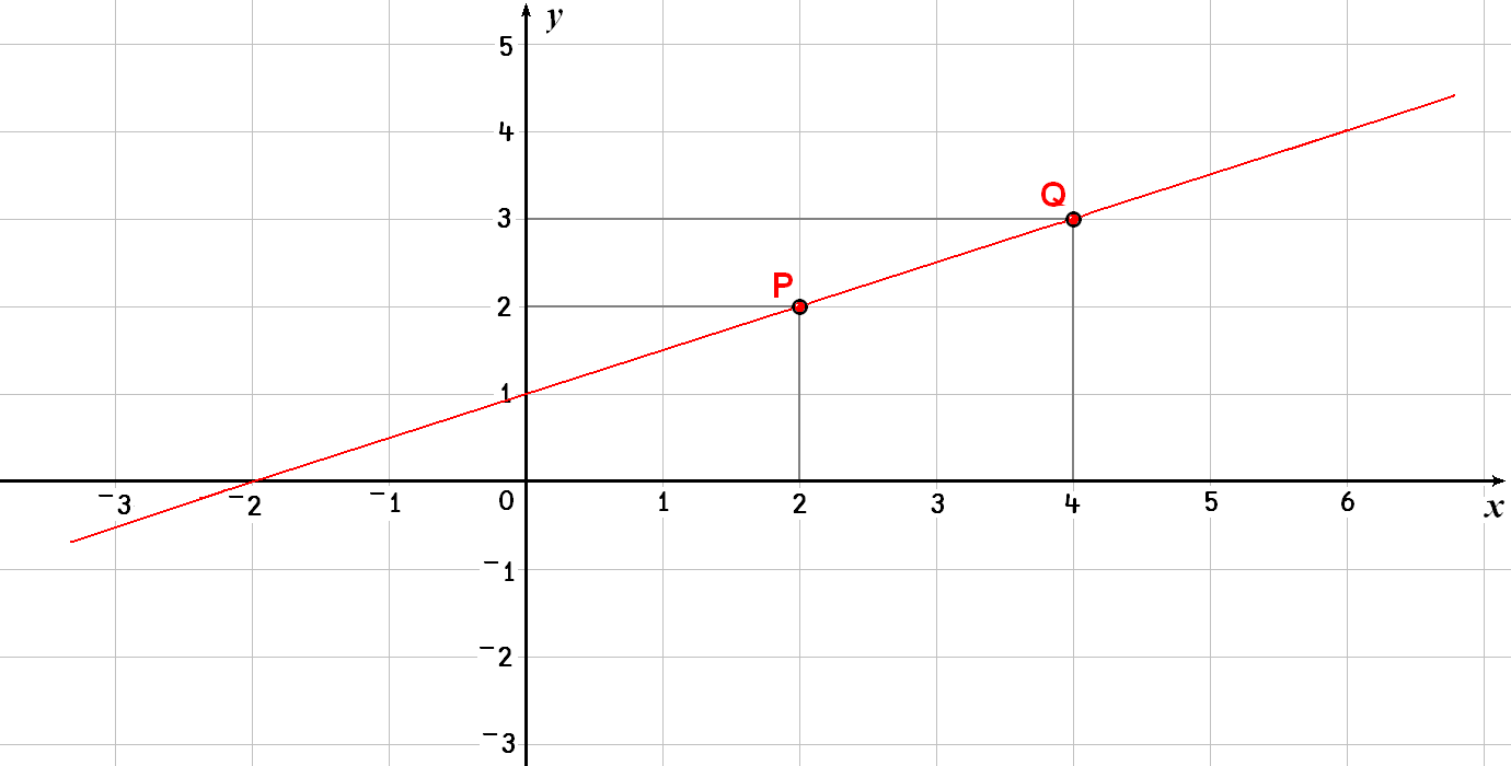
Fig. 13.1 A graph with the points P and Q.#
The general equation describing a straight line is \(y = mx + b\). With our two points given, the following is obtained:
This is a set of two linear equations in which the unknowns are \(m\) and \(b\). Let us solve this set of equations by the method demonstrated in the previous section:
cons ← ys
⎕← coefs ← xs,[1.5]1
Now, \(m\) and \(b\) can be calculated using the method we saw above:
⎕← c ← cons⌹coefs
We can also compute the coefficients of the line directly from the vectors xs and ys:
⎕← c ← ys⌹xs,[1.5]1
In traditional notation, this gives us the equation \(y = 0.5x + 1\) for the line. Did you find this tedious? Maybe, but now let us discover its scope.
13.5.4.2. Calculating Additional Y Coordinates#
Having found the coefficients of the line shown in the previous section, let us try to calculate the y coordinates of several points for which the x coordinates are known.
The coefficients of our line were obtained by this calculation:
c ← ys⌹coefs
We saw earlier that this is strictly equivalent to c ← (⌹coefs) +.× ys.
Let us multiply both terms of this expression by coefs:
             c ≡ (⌹coefs) +.× ys ←→
←→ coefs +.× c ≡ coefs +.× (⌹coefs) +.× ys ←→
←→ coefs +.× c ≡ ys
This shows that the y coordinates ys of some points placed on a line defined by the coefficients c can be calculated from their x coordinates xs by the formula coefs +.× c or, in a more explicit form: ys ← c +.×⍨ xs,[1.5]1.
Let us apply this technique to a set of points:
c +.×⍨ 0 ¯2 3 6,[1.5]1
You can check these values in Fig. 13.1.
13.5.5. Least Squares Fitting#
13.5.5.1. Linear Regression#
Our line was defined by two points. What happens if we no longer have 2 points, but many? Of course, there is a high probability that these points are not aligned.
As an example, suppose that we have twelve employees and we know their ages (in years) and salaries (in peanuts):
age ← 20 21 28 31 33 34 36 37 40 44 45 51
salaries ← 3071 2997 2442 3589 3774 3071 3108 5291 5180 7548 5772 5883
age,[.5]salaries
We shall place the ages on the x axis and salaries on the y axis (see Fig. 13.2).
This time, the matrix
age,[1.5]1
will have more rows (12) than columns (2), and the set of equations has no solution, which confirms that no single straight line can join all those points.
In this type of situation, it may be desirable to define a straight line which best represents the spread of points. Generally, a straight line is sought such that the sum of the squares of the deviations of the y coordinates between the given points and the line is minimised. This particular line is called the least squares line and the process of finding it is called linear regression.
To find this line, we shall use ⌹ once more.
The expression used to calculate the coefficients of a line passing through two points can be applied to a rectangular matrix, and the function matrix divide gives the coefficients of the least squares line passing through the set of points.
Is it not magic?
For the given points, here is the calculation:
⎕← c ← salaries⌹age,[1.5]1
This gives the line \(y = 134.946x - 412.6\).
We can calculate the approximate salaries located on the line, at the same x coordinates as the given points and compare with the actual salaries:
0⍕ salaries ,[.5] c+.×⍨age,[1.5]1
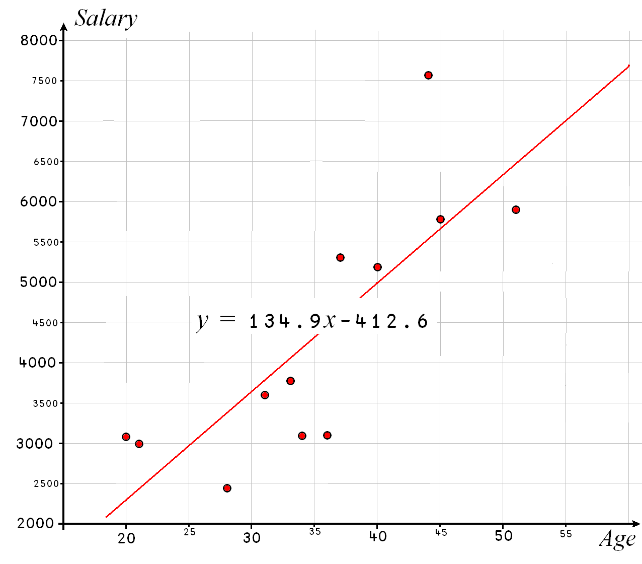
Fig. 13.2 Graph with the salaries (in peanuts) as a function of the age#
13.5.5.2. Extension#
In the previous example, we measured the effect of a single factor (age) on a single observation (salary) using a linear model.
What if we want to use the same model to explore the relationship between several factors and a single observation? The following example is inspired by a controller in IBM France who tried to see if the heads of his commercial agencies had “reasonable” expense claim forms.
The amounts were stored in a vector amounts.
He tried to measure the effect of 4 factors on these expenses amounts:
the number of salesmen in each agency,
nbmen;the size of the area covered by each agency,
radius;the number of customers in each agency,
nbcus; andthe annual income produced by each agency,
income.
In other words, he tried to find the vector tc of 5 theoretical coefficients, \(c_1, \cdots, c_5\), which most closely satisfy this equation:
Or, in APL, we want to find the 5-element vector tc that most closely satisfies this equality:
amounts ≡ tc +.× nbmen radius nbcus income 1
Here is the data:
amounts ← 40420 23000 28110 32460 25800 33610 61520 44970
nbmen ← 25 20 24 28 14 8 31 17
radius ← 90 50 12 12 30 30 120 75
nbcus ← 430 87 72 210 144 91 207 161
income ← 2400 9000 9500 4100 6500 3300 9800 4900
Let us apply exactly what we did on ages and salaries, and calculate the following variables:
⎕← coefs ← nbmen,radius,nbcus,income,[1.5]1
Next, we compute the 5 coefficients of the least squares line:
⎕← 2⍕tc ← amounts⌹coefs
Now, we compute the y coordinates of the points on the least squares line:
ys ← coefs+.×tc
Finally, we compute the differences between the expenses predicted by the expenses claims and the actual claims, and we compute the percentage deviation:
diff ← amounts-ys
pcent ← 100×diff÷ys
Finally, we display all the data, with a “-” next to the agencies for which the expenses are significantly above the predicted value (possibly because the agencies have bad managers) and a “+” sign next to the agencies for which the expenses are significantly below the predicted value (possibly because the agencies have good managers):
⎕← flag ← '+ -'[1+¯10 10⍸pcent]
⎕← title ← 29↑' Real Normal Diff %'
title⍪(7 0⍕amounts,ys,diff,[1.5]pcent),flag
13.5.5.3. Non-linear Adjustment#
In this last example we used independent factors and tried to combine them with a linear expression.
We could as well have used vectors linked one to the other by any mathematical expression, like results ← (c1×var)+(c2×var*2)+(c3×⍟var)+c4 (if this makes sense).
A typical case is trying to fit a set of points with a polynomial curve.
Here are 8 points:
xs ← ¯1 ¯1 0.5  1.5  2 2 3 4
ys ← ¯3 ¯1 0   ¯1   ¯1 1 3 5
A linear regression would give a line with the following coefficients:
2⍕ ys⌹xs,[1.5]1
The right argument was obtained by laminating 1 to xs.
However, we could just as well have obtained it with the following outer product:
xs∘.*1 0
Now, instead of taking only powers 1 and 0 of xs, we could extend the scope of the powers up to the third degree, for example:
xs∘.*3 2 1 0
We would then obtain not the coefficients of a straight line, but those of a third degree polynomial curve, shown in Fig. 13.3.
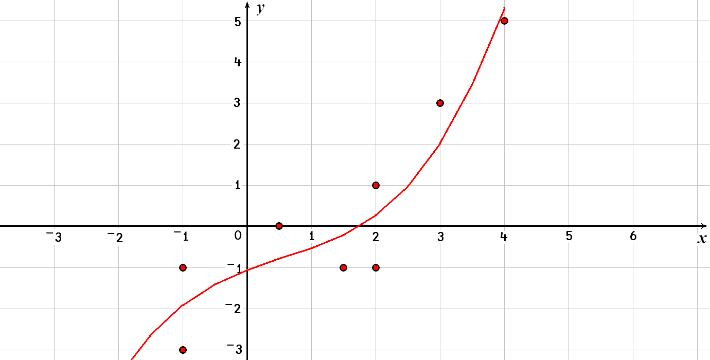
Fig. 13.3 A third degree polynomial adjusted to some points.#
To get the coefficients, we do the usual computation:
2⍕ c←ys⌹xs∘.*3 2 1 0
In other words, this set of points can be approximated by the line \(0.1x^3 - 0.16x^2 + 0.58x - 1.07\).
13.6. Exercises#
Exercise 13.1
Can you predict (and explain) the results of the two expressions below?
0 ⊥ 12 34 60 77 19
1 ⊥ 12 34 60 77 19
Exercise 13.2
In a binary number system, a group of 4 bits represents values from 0 to 15. Those 4 bits represent the 16 states of a base 16 number system known as the hexadecimal number system. This system is very often used in computer science, with the numbers 0-9 represented by the characters “0”-“9”, and the numbers 10-15 represented by the characters “A” to “F”. Write a function to convert hexadecimal values to decimal, and the reverse. Assume hexadecimal values are represented as 4 character vectors:
D2H ← {'0123456789ABCDEF'[1+16 16 16 16⊤⍵]}
(⍪,D2H¨) ¯1+⍳16
D2H¨ 6748 49679 60281
H2D ← {16⊥¯1+'0123456789ABCDEF'⍳⍵}
H2D¨ '1A5C' 'C20F' 'EB79'
Exercise 13.3
A sparse array is an array of zeroes with only a small number of non-zero elements.
To save memory, sparse arrays are often represented in condensed forms, where we only store the positions of the non-zero values.
In this exercise, you will write two functions, Contract and Expand, to convert a sparse array into its compressed form and vice-versa.
Contract accepts an arbitrary sparse array sa as its only argument and returns a vector with the following characteristics:
the first element is the rank
rofsa;the next
relements are the shape ofsa;the next
nelements are thennon-zero values ofsa; andthe final
nelements are the positions of the corresponding non-zero elements. However, the finalnelements should be the indices of the non-zero values in the ravel ofsa, and not the high-rank indices.
The function Expand should do the reverse operation.
Implement Contract and Expand without using the function ravel.
Here is a worked example with a 5 by 7 matrix:
sa ← 5 7⍴0 ⋄ sa[1;2] ← 3 ⋄ sa[4;1] ← 5.6
⎕← sa
]dinput
Contract ← {
    flat ← 1+(⍴⍵)⊥¯1+⍉↑idx←⍸0≠sa
    (≢⍴⍵),(⍴⍵),⍵[idx],flat
}
Contract sa
The matrix sa has two non-zero values at indices 1 2 and 4 1, respectively.
However, in the ravel of sa, those two non-zero values are at indices 2 and 22:
(,sa)[2 22]
Thus, the final part of the result of Contract sa should be the 4-item vector 3 5.6 2 22:
      Contract sa
2 5 7 3 5.6 2 22
↑ ~~~ ∧∧∧∧∧ ∧∧∧∧
| |   |   the corresponding indices are 2 and 22
| |   the non-zero values are 3 and 5.6
| shape of sa
rank of sa
The function Expand should do the reverse operation:
Exercise 13.4
Create three variables, filled with random integers, according to the following specifications:
a vector of 12 values between 8 and 30, without duplicates;
a 4 by 6 matrix filled with values between 37 and 47, with possible duplicates; and
a 5 by 2 matrix filled with values between ¯5 and 5, without duplicates.
Exercise 13.5
Create a vector of 15 random numbers between 0.01 and 0.09 inclusive, with 3 significant digits each, with possible duplicates.
Exercise 13.6
What will we obtain by executing the expression 10+?(10+?10)⍴10?
Exercise 13.7
We would like to obtain a vector of 5 items, chosen randomly and without duplicates among the elements of list ← 12 29 5 44 31 60 8 86.
Exercise 13.8
Create a vector with a length randomly chosen between 6 and 16, and filled with random integers between 3 and 40 inclusive, with possible duplicates.
Exercise 13.9
The value of \(\cos x\) can be calculated by the following formula, written with traditional mathematical notation:
Write a function n Cos x that accepts an integer n as left argument and a value x as right argument and computes the value of the expression above up to the power 2×n, for the value x.
(To verify your answer, n Cos x should be close to 2○x.)
Exercise 13.10
Try to evaluate the following expressions, and then check your result on the computer:
(1○○÷4)*2; and2×0.5+¯2○1○0.5.
(This exercise assumes you have some trigonometry knowledge.)
Exercise 13.11
Find the solution to this set of equations:
Exercise 13.12
Three variables \(a\), \(b\), and \(c\), meet the following conditions:
Can you calculate the value of \(3a + 5b - c\)?
13.7. The Specialist’s Section#
You will find here rare or complex usages of the concepts presented in this chapter, or discover extended explanations which need the knowledge of some symbols that will be seen much further in the book.
If you are exploring APL for the first time, skip this section and go to the next chapter.
13.7.1. Advanced Encode and Decode#
13.7.1.1. Special Decoding#
If you replace decode by the equivalent inner product, you can easily check these surprising properties:
0⊥v ←→ ⍬⍴¯1↑v
1⊥v ←→ +/v
When dealing with integers, the values are normally smaller than the corresponding items of the base. For example, it would be unusual to say that a time is equal to 7 hours, 83 minutes, and 127 seconds. However, decode works perfectly on such values:
24 60 60 ⊥ 7 83 127
And, though we did not mention it, encode (like decode) accepts decimal and/or negative bases:
3⍴5.2 ⊤ 160.23
13.7.1.2. Processing Negative Values#
Imagine that we want to encode some numbers in any base, with 6 digits. We will choose base 10, so that the result is readily understandable:
(6⍴10)⊤17
Now, let us try to predict the result of (6⍴10)⊤¯17.
Knowing that 17+¯17 is 0, it would be reasonable to expect that ((6⍴10)⊤17)+((6⍴10)⊤¯17) also returns a result that is “zero” in some way – for example 6⍴0?
In other words, we are looking for a 6-item vector that, when added to 0 0 0 0 1 7, gives 6⍴0.
The real challenge is that the items of the vector must only contain the digits 0 through 9!
Let us see what happens:
(6⍴10)⊤¯17
These results may seem a bit surprising.
In base 10, when the sum of two digits exceeds 9, a carry is produced, which is used when adding the next digits to the left, and so on.
When adding the encoded values of 17 and ¯17, here is how the values are processed:
  1 1 1 1 1 1
    0 0 0 0 1 7
+   9 9 9 9 8 3
  -------------
= 1 0 0 0 0 0 0
If only 6 digits are kept, as agreed, you can see that the result is composed only of zeroes (the six leftmost digits in the result).
That would be the same for 431 and ¯431:
(6⍴10)⊤431
(6⍴10)⊤¯431
We can observe the same behaviour in any other base. For example, in base 5:
(6⍴5)⊤68
(6⍴5)⊤¯68
Remember that, in base 5, 0=3+2!
The rule remains true for decimal values:
(6⍴10)⊤15.8
(6⍴10)⊤¯15.8
This may lead to a few frustrations during decoding if precautions are not taken:
10⊥(6⍴10)⊤ 143 ⍝ as expected
10⊥(6⍴10)⊤¯143 ⍝ this may seem wrong
The result obtained from the two decodings is such that their sum is 1,000,000.
If one needs to encode and later decode values among which some may be negative, it is advisable to provide one more digit than is necessary, and to test its value. In many computers, the internal representation of positive numbers begin with a 0-bit and negative numbers start with a 1-bit. The same principle applies to the decoded values. In base 10, positive values begin with the digit 0, and negative ones with a 9. From this, we can deduce a general function to decode values encoded in a uniform base:
]dinput
Decode ← {  ⍝ base Decode values
    z ← ⍺⊥⍵
    p ← 1↑⍴⍵
    z-(⍺*p)×(z>¯1+⍺*p-1)
}
test ← (6⍴10) ⊤ ¯417.42 26 32 ¯1654 0 3.7 ¯55
10⊥test ⍝ negative values are wrongly decoded...
10 Decode test ⍝ positive values are correctly decoded!
13.7.1.3. Multiple Encoding/Decoding#
It is possible to decode a value using several bases simultaneously:
⎕← bb ← ⍉4 3⍴5 10 6
The different bases are placed in different rows of the matrix.
Now, we can interpret 4 1 3 2 in 3 different bases:
bb⊥4 1 3 2
In this very specific case, the 3 bases were all uniform; a simple column vector with one digit per row would have given the same conversion:
(⍪5 10 6)⊥4 1 3 2
That is because a scalar base expands into as many digits as needed.
Similarly, it is possible to see how a single number could be represented in several bases:
(5 3⍴5 10 2)⊤27
Remark
The arguments of encode and decode must obey the following rules:
In
r ← bases ⊥ mat,⍴ris equal to(¯1↓⍴,bases),1↓⍴mat.In
r ← bases ⊤ mat,⍴ris equal tobases ,⍥⍴ mat.
Let us convert (encode) the following matrix seconds into hours, minutes, and seconds:
⎕← seconds ← 2 3⍴1341 5000 345 3600 781 90
24 60 60 ⊤ seconds
The first plane of the 3D array contains the hours, the second plane contains the minutes, and the third plane contains the seconds.
13.7.2. Gamma and Beta Functions#
In mathematics, the gamma function of a variable \(x\) is defined by the following formula:
This function satisfies the recurrence relationship \(\Gamma(x) = x\times \Gamma(x-1)\).
If \(x\) is an integer, \(\Gamma(x)\) is the same as \((x-1)!\).
In APL, monadic !n gives the gamma function of n+1:
! 2.4 3 3.2 3.4
The dyadic form of ! gives the binomial function, which satisfies the following identity with the mathematical beta function: \(\beta(a, b)\) is identical to ÷b×(a-1)!a+b-1.
13.7.3. Domino and Rectangular Matrices#
We have defined the matrix inverse for square matrices, but throughout this chapter we have used the function matrix divide on rectangular matrices. In the following sections we shall define what are the “left inverse” and the “right inverse” of a given rectangular matrix.
Remark
Under the hood, domino uses Householder transformations, a technique based on the Lawson & Hanson algorithm, an extension of the Golub & Businger algorithm.
13.7.3.1. Left Inverse of a Matrix#
We have been working in this context:
yswas a vector of values we wanted to predict.coefswas a rectangular matrix containing a set of columns containing variables (for example, number of salesmen, size of the area, number of customers, …).ccontained the coefficients of the least squares line. They should be such that the sum of the squares of the differences between points on this line and the given points inysis minimal.
In mathematics, three major properties can be demonstrated:
The coefficients
ccan be obtained fromysby means of a linear regression or, in other words, an inner product involving a matrixinv:c ← inv+.×ys.This matrix
invis unique.It can be obtained by the following formula:
inv ← (⌹ (⍉coefs)+.×coefs)+.×⍉coefs.
In this formula, the product (⍉coefs)+.×coefs gives a square matrix, even if coefs is rectangular.
This is why we can calculate its inverse using the function matrix inverse.
If we refer to the definition of matrix divide, (⌹a)+.×b can be written as b⌹a.
So, the formula for inv can be rewritten as inv ← (⍉coefs)⌹(⍉coefs)+.×coefs.
Let us see what happens if we multiply that formula by coefs on the right:
   inv ≡ (⌹ (⍉coefs)+.×coefs)+.×⍉coefs ←→
←→ inv +.× coefs ≡ (⌹ (⍉coefs)+.×coefs)+.×⍉coefs +.× coefs
Now, if we define U ← (⍉coefs)+.×coefs, we see that the expression above actually reads
inv +.× coefs ≡ (⌹U)+.×U
(⌹U)+.×U is the identity matrix, so we actually see that inv is a left inverse of coefs, because if we multiply coefs with inv on the left, we get the identity matrix.
Rule
The left inverse of a matrix m can be computed with (⌹(⍉m)+.×m)+.×⍉m.
This can be easily verified with the data we used in a previous example:
coefs
inv ← (⌹(⍉coefs)+.×coefs)+.×⍉coefs
⌊0.5+inv+.×coefs
Once rounded, we can see it is an identity matrix and inv really is a left inverse of coefs.
13.7.3.2. Pseudo Right Inverse#
We just saw that inv is a left inverse for coefs.
Is it also a right inverse?
We calculated the coefficients in c of the least squares line using the formula c←inv+.×ys.
Then, we calculated the coordinates of points located on that line with fits ← coefs+.×c.
Let us replace c by its definition from the first formula, to get fits ← coefs+.×inv+.×ys.
If inv was a true right inverse of coefs, the product coefs+.×inv would give the identity matrix and the product coefs+.×inv+.×ys would evaluate to ys.
However, we know that ys≢fits in general, because coefs+.×inv+.×ys gives the predicted values on top of the line, whereas ys contains the actual values we are trying to fit the line to.
The difference between fits and ys is such that +/(ys-fits)*2 is minimised.
In the expression ys-fits, let us replace fits by coefs+.×inv+.×ys and then replace ys by I+.×ys (I is the identity matrix, so this does not change anything) to get (I+.×ys) - (coefs+.×inv+.×ys).
Using ys as a common factor, this can be rewritten as (I-coefs+.×inv)+.×ys.
If +/(ys-fits)*2 is minimised, +/((I-coefs+.×inv)+.×ys)*2 should be minimised too.
This must be true whatever the value of ys, including the case where ys is 1.
This means that the value of inv (calculated independently of ys) is such that it minimised the expression +/(I-coefs+.×inv)*2.
We can say that inv is a pseudo right inverse matrix of coefs that minimises +/(I-coefs+.×inv)*2.
In APL, matrix inverse has been extended to calculate such a pseudo inverse: inv ← ⌹coefs.
13.7.3.3. Summary of Left and Right Inverses#
In APL, a matrix M having more rows than columns has an inverse, which can be obtained by ⌹M.
This inverse value is strictly equal, within rounding errors, to any of the following formulas:
      inv ← (⌹(⍉M)+.×M)+.×⍉M
      inv ← (⍉M)⌹(⍉M)+.×M
This matrix is a true left inverse of M, which means that the product inv +.× M gives an identity matrix.
This matrix is also a pseudo right inverse of M.
That is to say that the product does not give an identity matrix, but a matrix J such that the sum +/(I-J)*2 is minimised.
the result of this is to minimise any expression of the form +/((I-M+.×inv)+.×ys)*2, whatever the value of ys.
This last property explains why domino may be used to calculate linear, multi-linear, or polynomial regressions.
13.7.3.4. Scalars and Vectors#
A scalar s is treated in such a way that ⌹s is equal to ÷s with the exception that 0÷0 is 1 whereas 0⌹0 gives a DOMAIN ERROR.
Vectors are treated like single-column matrices:
⎕← cv ← ⌹v ← 2 ¯1 0.5
cv +.× v
v +.× cv
13.7.4. Total Array Ordering#
In Dyalog, there is something called total array ordering, used by the functions grade up and down and interval index. In the earlier days of Dyalog APL, only simple arrays of the same shape and type could be compared. Thus, by introducing total array ordering, APL can now order simple and nested arrays of any rank, shape, and type.
Total array ordering is very nuanced. For example, all numbers come before characters:
⍋3 '3'
⍋234562345243 '3'
⍋0J1 '3'
Complex numbers can also be ordered with other numbers:
⍋¯2J¯1 ¯1J¯3 0 0J4 3
However, mathematics tells us that there is no “natural ordering” for the complex numbers. This means that we cannot order the complex numbers in a way that preserves the properties of addition and multiplication that we are used to.
For example, a negative number times a positive number yields a negative number. Recall that “negative” really means “less than zero” and “positive” means “greater than zero”. Below, we can see two complex numbers, one less than zero and the other greater than zero:
⍋¯2J1 0 1J¯2
The product of the two complex numbers shown above is:
1J¯2 × ¯2J1
And the product is greater than zero:
⍋0 0J5
We can see that complex numbers are ordered by real part and then by imaginary part:
⍋¯2J¯100 ¯2 ¯2J1 0J¯7654321 0 0J1 3
Total array ordering also allows the ordering of nested and mixed arrays:
⍋ ⎕← (⊂⊂⊂0J1 '0J2') 5 ('a',⍳3) ('hey' ('bye' 1 2 (3 'ciao')))
In Dyalog APL, the only simple scalars that are considered by the total array ordering are nulls, numbers, and characters. In other words, total array ordering does not contemplate namespaces, objects, and object representations.
For example, the following usage of grade up fails because of the namespace in the vector:
⍋1 2 (⎕NS⍬) 4
DOMAIN ERROR
      ⍋1 2(⎕NS ⍬)4
      ∧
Fig. 13.4 A man holding a blue hammer chasing a piggy bank.#
13.8. Solutions#
Solution to Exercise 13.1
We know that n ⊥ 12 34 60 77 19 is equivalent to n n n n n ⊥ 12 34 60 77 19, whatever the value of n.
Furthermore, we saw that the weights used in the conversion are given by the expression ⌽1,×\⌽1↓n n n n n.
So, if n ← 0, we get that the weights are
⌽1,×\⌽1↓5⍴0
This means that the 19 is multiplied by 1 and everything else by 0, so the final result is 19:
0 ⊥ 12 34 60 77 19
Therefore, 0⊥vec gives the last element of a numeric vector.
If n ← 1, the weights are
⌽1,×\⌽1↓5⍴1
This means that every number is multiplied by 1, and thus 1⊥ gives the sum of a vector:
1 ⊥ 12 34 60 77 19
+/ 12 34 60 77 19
Solution to Exercise 13.2
Because we know that hexadecimal values will take up 4 characters only, we can safely do 16 16 16 16⊤⍵ to encode a decimal number to base 16:
D2H ← {'0123456789ABCDEF'[1+16 16 16 16⊤⍵]}
(⍪,D2H¨) ¯1+⍳16
D2H¨ 6748 49679 60281
If we did not know how long the hexadecimal number would be, we could use 16⊥⍣¯1⊢ instead:
{'0123456789ABCDEF'[1+16⊥⍣¯1⊢⍵]} 123456789
H2D ← {16⊥¯1+'0123456789ABCDEF'⍳⍵}
H2D¨ '1A5C' 'C20F' 'EB79'
Solution to Exercise 13.3
Let us work through the solution with the example of the matrix sa:
sa ← 5 7⍴0 ⋄ sa[1;2] ← 3 ⋄ sa[4;1] ← 5.6
⎕← sa
To implement the function Contract, we need to find the non-zero values of sa and their indices:
sa[idx ← ⍸0≠sa]
idx
Now, we need to decode these multidimensional indices into the one-dimensional indices of the ravel, which we can do with the function decode and the shape of the array (sa, in our example).
However, indexing is 1-based and encode and decode start counting from 0, so we need to subtract 1 from the indices in the beginning and add 1 at the end:
1+(⍴sa)⊥¯1+⍉↑idx
We can verify these indices are correct:
(,sa)[2 22]
Now, we can put Contract together:
]dinput
Contract ← {
    flat ← 1+(⍴⍵)⊥¯1+⍉↑idx←⍸0≠⍵
    (≢⍴⍵),(⍴⍵),⍵[idx],flat
}
⎕← compressed ← Contract sa
To implement Expand, we work in the other direction.
We start by finding the rank and the shape of the original sparse array:
⎕← rank ← ⊃compressed
⎕← shape ← rank↑1↓compressed
⎕← rest ← compressed↓⍨1+rank
Now, we need to split the remainder into the values and the indices:
⎕← values ← rest↑⍨0.5×≢rest
⎕← idx ← rest↓⍨0.5×≢rest
Now, we use encode and the shape of the array to transform the linear indices into the multidimensional ones:
↓⍉1+shape⊤¯1+idx
]dinput
Expand ← {
    shape ← (⊃⍵)↑1↓⍵
    rest ← ⍵↓⍨1+⊃⍵
    values ← rest↑⍨0.5×≢rest
    idx ← rest↓⍨0.5×≢rest
    arr ← shape⍴0
    arr[↓⍉1+shape⊤¯1+idx] ← values
    arr
}
Expand compressed
As another example, here is a cuboid with five non-zero elements:
cuboid ← 3 7 21⍴0
cuboid[(,⍳⍴cuboid)[5?×/⍴cuboid]] ← ⍳5
cuboid
cuboid ≡ Expand Contract cuboid
Solution to Exercise 13.4
a vector of 12 values between 8 and 30, without duplicates:
7+12?23
a 4 by 6 matrix filled with values between 37 and 47, with possible duplicates:
36+?4 6⍴11
a 5 by 2 matrix filled with values between ¯5 and 5, without duplicates:
¯6+5 2⍴10?11
Solution to Exercise 13.5
0.0001×99+?15⍴801
Solution to Exercise 13.6
The expression starts with (10+?10)⍴10 which will create a vector filled with 10, with a random length between 11 and 20.
Then, the final 10+?... will generate random integers between 1 and 10 and add 10 to those, so the final result is a vector of a random length between 11 and 20 with random elements between 11 and 20.
10+?(10+?10)⍴10
10+?(10+?10)⍴10
10+?(10+?10)⍴10
Solution to Exercise 13.7
list ← 12 29 5 44 31 60 8 86
list[5?⍴list]
Solution to Exercise 13.8
2+?(5+?11)⍴38
Solution to Exercise 13.9
Cos ← {(⍵*p)-.÷!p←2×0,⍳⍺}
2○○1
10 Cos ○1
Solution to Exercise 13.10
(1○○÷4)*2:
\(\sin \pi/4 = \sqrt{\frac12}\), thus the square of that is 0.5:
(1○○÷4)*2
2×0.5+¯2○1○0.5:
¯2○1○0.5 is \(\arccos(\sin \frac12)\), which is \(\frac\pi2 - \frac12\), so the whole expression evaluates to \(\pi\):
2×0.5+¯2○1○0.5
○1
Solution to Exercise 13.11
We can solve this set of linear equations with the function matrix divide. We just need to be careful when writing the matrix of coefficients.
5 ¯7 2⌹3 3⍴1 ¯1 0 0 1 ¯2 ¯1 0 1
Solution to Exercise 13.12
To compute the value of \(3a + 5b - c\), the easiest thing to do is to start by finding the values of \(a\), \(b\), and \(c\), which we can do by solving the set of linear equations:
⎕← (a b c) ← abc ← 13 ¯6 10⌹3 3⍴1 ¯1 3 ¯2 4 0 1 ¯2 2
Finally, we can compute the value of that expression in a couple of ways:
(3×a)+(5×b)-c
abc+.×3 5 ¯1
We could have done this computation directly:
3 5 ¯1+.×13 ¯6 10⌹3 3⍴1 ¯1 3 ¯2 4 0 1 ¯2 2