Execute & Format Control
Contents
7. Execute & Format Control#
7.1. Execute#
7.1.1. Definition#
Execute is a monadic function represented by ⍎, which you can type with APL+;; its dyadic use will be explained in the Specialist’s Section at the end of this chapter.
Execute takes a character vector (or scalar) as its argument.
If the character vector represents a valid APL expression, Execute will just… execute it, as if it had been typed on the keyboard. Otherwise, an error will be reported.
Take a look at the following example:
⎕← letters ← '5×6+2'
⍎letters
The argument can contain any valid expression:
numeric or character constants, or variables;
left arrows (assignment) or right arrows (branch);
primitive or defined functions and operators; and
calls to other execute functions.
Let us define a short function to call from within execute:
∇ r ← x Plus y
    r ← x + y
∇
In the expression below, execute calls our Plus function and creates a new variable:
⍎'new ← 3 + 4 Plus 5'
new
If the expression returns a result, it will be used as the result of execute:
res ← ⍎'3 Plus 10'
res
We could just as well have written
⍎'res ← 3 Plus 10'
res
Beware
Note that if the argument does not return a result, it can still be executed, but execute will not return a result, and any attempt to assign it to a variable or to use it in any other way will cause a VALUE ERROR.
Take a modification of our Plus function that returns no result:
∇ x PlusNoRes y;r
    r ← x+y
∇
These expressions all work:
⍎''
⍎'     '
⍎'3 PlusNoRes 5'
But trying to assign results from all those expressions will fail,
res ← ⍎''
res ← ⍎'     '
res ← ⍎'3 PlusNoRes 5'
VALUE ERROR: No result was provided when the context expected one
      res←⍎''
          ∧
VALUE ERROR: No result was provided when the context expected one
      res←⍎'     '
          ∧
⍎VALUE ERROR: No result was provided when the context expected one
      3 PlusNoRes 5
        ∧
because that is equivalent to writing the following:
res ←
res ←
res ← 3 PlusNoRes 5
SYNTAX ERROR: Missing right argument
      res←
         ∧
SYNTAX ERROR: Missing right argument
      res←
         ∧
VALUE ERROR: No result was provided when the context expected one
      res←3 PlusNoRes 5
            ∧
7.1.2. Some Typical Uses#
7.1.2.1. Convert Text into Numbers#
Execute may be used to convert characters into numbers.
One common application of execute is to convert numeric data, stored as character strings in a text file (for example, a .csv file), into binary numbers.
You can just read in a string such as '123, 456, 789' and execute it to obtain the corresponding 3-item vector:
⍎'123, 456, 789'
We saw in the chapter about user-defined functions that format can be used to convert numbers to characters; the reverse can be done using execute. This explains why those two functions are represented by “reversed” symbols, as shown in Fig. 7.1:
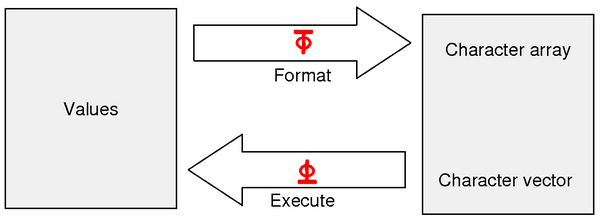
Fig. 7.1 Representation of the duality between the execute and format primitives.#
There is, however, a major difference: format can be applied to matrices, whereas execute can only be applied to vectors.
birthdate ← 'October 14th, 1952'
+/ ⍎ ⎕←birthdate[9 10,13+⍳5]
Notice that the '14 1952' above is a character vector of length 7, and not a vector of 2 character vectors.
In fact, compare
birthdate[9 10,13+⍳5]
≢birthdate[9 10,13+⍳5]
with
'14' '1952'
to which ⍎ cannot be applied:
⍎'14' '1952'
DOMAIN ERROR
      ⍎'14' '1952'
      ∧
Because execute can only be applied to vectors, a matrix of numeric characters can only be converted after it has been ravelled. But to avoid characters of one row being attached to those of the previous row, it is necessary to catenate a blank character before ravelling.
As an example, take the matrix mat below:
⎕← mat ← 4 4⍴' 8451237 9332607'
If we ravel it and execute it, we get
⍎,mat
which is not what we want. The correction conversion will be obtained by first catenating a blank space:
⍎,mat,' '
7.1.2.2. A Safer and Faster Solution#
Using execute to convert characters into numbers may cause errors if the characters do not represent valid numbers.
So, we strongly recommend that you instead use ⎕VFI (for Verify and Fix Input).
This is a specialised system function that performs the same conversion, but securely, and is about twice as fast as execute.
⎕VFI will be studied in the chapter about system interfaces.
7.1.2.3. Other Uses#
Execute can be used for many other purposes, including some that may be considered to be rather advanced programming techniques. Some examples are provided in the Specialist’s Section at the end of this chapter:
conditional execution (rather obsolete);
case selection (also obsolete);
dynamic variable creation.
Please bear in mind that these execute use-cases aren’t necessarily recommended programming practices.
7.1.3. Make Things Simple#
The vector passed in to execute is often constructed by catenating pieces of text, or tokens.
These tokens may contain quotes (which must then be doubled), commas, parentheses, etc. But to build the final expression, you will also need quotes (to delimit the tokens), commas (to concatenate them), parentheses, and so on.
By now, the expression is becoming extremely complex. It may be difficult to see if a comma is part of a token or is being used to concatenate two successive tokens, and this is only partly alleviated by syntax colouring that modern IDEs provide. It may be hard to see whether or not the parentheses and quotes are properly balanced. If the final expression is wrong, fixing it might be difficult, and if it is correct, later modifying it or expanding it might be just as difficult.
To simplify maintenance, it is good practice to assign the text to a variable before executing it. If the operation fails, for any reason, you can just display the variable to see if it looks correct. For example, here is a statement involving execute:
size ← 43
⍎'tab',(⍕size),'←(4 ',(⍕size),'⍴'') '''
⍎SYNTAX ERROR: Unpaired parenthesis
      tab43←(4 43⍴') '
            ∧
That’s rather obscure! If any problem occurs, it can be difficult to spot the cause.
Let us insert a variable just before the execute function:
⍎debug←'tab',(⍕size),'←(4 ',(⍕size),'⍴'') '''
⍎SYNTAX ERROR: Unpaired parenthesis
      tab43←(4 43⍴') '
            ∧
Now, it easy to look at debug and see if its value is what we would expect:
debug
Obviously, this is not a correct statement, so it failed when we tried to execute it.
7.2. The Format Primitive#
The format primitive function ⍕, typed with APL+’, has already been briefly described in Section 5.9.2.
We shall cover it in more depth in this section.
7.2.1. Monadic Format#
Monadic format converts any array, whatever its value, into its character representation.
This applies to numbers, characters, and nested arrays.
The result is exactly the same as you would see if you displayed the array on your screen, because APL internally uses monadic format to display arrays.
The previous statement assumes that you have no options modifying your output; for example, if you have ]box on it is no longer true that format produces exactly the same representation as if you just displayed the the array yourself:
⍕1 (2 3)
]box
1 (2 3)
Ignoring the effects of such session modifiers like ]box, which will be covered with some more detail later in this chapter (see Section 7.4.2), monadic format is such that:
character arrays are not converted, they remain unchanged; and
numeric and nested arrays are converted into vectors or matrices of characters.
⎕←chemistry ← 3 5⍴'H2SO4CaCO3Fe2O3'
chemistry is a character matrix with shape 3 5, and it is not modified by ⍕:
⍴⎕←⍕chemistry
chemistry≡⍕chemistry
On the other hand, a numeric vector with, say, 3 items, becomes a (longer) character vector once converted:
≢52 69 76
≢⎕←⍕52 69 76
A nested matrix like nesMat,
⍴⎕←nesMat ← 2 3 ⍴ 'Dyalog' 44 'Hello' 27 (2 2 ⍴ 8 6 2 4) (2 3⍴1 2 0 0 0 5)
which we have already used before, becomes a character matrix that is 20 characters wide and with 3 rows, because nesMat contained two small matrices:
⍴⎕←⍕nesMat
7.2.2. Dyadic Format#
7.2.2.1. Definition of Dyadic Format#
Dyadic format applies only to numeric values; any attempt to apply it to characters will cause a DOMAIN ERROR.
The general syntax of format is descriptor⍕values,
where values can be an array of any rank.
Dyadic format converts numbers into text in a format that is described by the left argument, the format descriptor.
descriptor is therefore made up of two numbers:
the first number indicates the number of characters to be assigned to each numeric value; or to put it another way, the width of the field in which each numeric value is to be represented; and
the second number indicates how many decimal digits will be displayed.
⎕RL ← 73
⎕←nm ← (?3 4⍴200000)÷100
The representation above is the normal display of the nm matrix, and it is also how monadic format would present the matrix.
Compare that with the result below, where we represent each number right-aligned in a field that is 8 characters wide, with 2 decimal digits.
8 2⍕nm
The result has, of course, 3 rows and 32 columns (8 characters for each of the 4 columns):
⍴8 2⍕nm
We can also draw a basic ruler (with the help of a short dfn) below the formatted matrix to help you count the width of each field:
]dinput
ruler ← {
    c ← ¯1↑⍴⍵
    ⍵⍪c⍴4 1 4 1/'¯''¯|'
}
ruler 8 2⍕nm
In the next example we represent each number in a field that is 6 characters wide, right-aligned, and with no decimal digits.
ruler 6 0⍕nm
The result has now 3 rows and 24 columns:
⍴6 0⍕nm
Remark
You can see that the numbers to be formatted are rounded rather than truncated when the specified format does not allow the full precision of the numbers to be shown.
7.2.2.2. Overflow#
If a column is not wide enough to represent some of the numbers, these numbers will be replaced by asterisks.
Recall what nm looked like:
nm
We have seen above that 8 2⍕nm looked good:
8 2⍕nm
If we reduce the width of the columns by 1, some values will now be adjacent to the values immediately to their left, making them difficult to read. For example, the second column will be adjacent to the left column:
7 2⍕nm
If we further reduce the width of the columns, the largest values will no longer fit in their allotted space and will be replaced by asterisks. Most of the other numbers are now adjacent to their neighbours.
6 2⍕nm
Remark
To calculate the width required to represent a number you must account for the minus sign, the integer digits, the decimal point, and as many decimal digits as specified in the descriptor.
7.2.2.3. Multiple Specifications#
One can define a different format for each column of numbers.
Each format definition is made of 2 numbers, so if the matrix has n columns, the left argument must have 2×n items:
ruler 8 2 10 0 9 4 8 2⍕nm
In this case, we formatted the first column with 8 2, the second column with 10 0, the third column with 9 4, and the fourth column with 8 2 again.
If the format descriptor (the left argument) does not contain enough pairs of values, it will be repeated as many times as needed, provided that the width of the matrix is a multiple of the number of pairs.
In other words, in desc⍕values, the residue (≢desc)|2ׯ1↑⍴values must be equal to 0, otherwise a LENGTH ERROR is reported.
For example,
desc ← 8 2 10 0
desc⍕nm
In the above, columns 3 and 4 reused the descriptors of columns 1 and 2, respectively 8 2 and 10 0.
This is equivalent to writing the repeated pairs by hand:
8 2 10 0 8 2 10 0⍕nm
We can also compare desc⍕nm with the statement above about the residue:
(≢desc)|2ׯ1↑⍴nm
7.2.2.4. Scientific Representation#
If the second item of a pair of format descriptors is negative, for example in 9 ¯3⍕12345, numbers are formatted in scientific notation (also described as exponential notation; see Section 3.10.2), with as many significant digits in the mantissa as specified by the descriptor:
8 ¯2⍕nm
8 ¯4⍕nm
You can refer to Wikipedia’s article on “Scientific Notation” for more information on how scientific notation works.
7.2.2.5. Scalar Descriptor#
When the descriptor is reduced to a simple scalar, the columns are formatted in the smallest width compatible with the values they contain, plus one separating space. The scalar descriptor is then used to specify the number of decimal places to use, or the number of significant digits to use in the mantissa of the scientific representation of the numbers, depending on the sign of the descriptor.
For example,
2⍕nm
tells ⍕ to use 2 decimal places for all numbers, whereas
¯3⍕nm
tells ⍕ to use 3 digits in the mantissa of all numbers.
In both examples above we see that each column is separated from the preceding one (and from the left margin too!) by a single space.
This technique is convenient for experimental purposes, to have the most compact presentation possible, but you cannot control the total width of the final result with it.
7.3. The ⎕FMT System Function#
The format primitive function is inadequate for producing professional looking output, such as one may require for common business purposes, because:
negative values are represented by a high minus sign, which is rather unusual outside the APL world;
a large value, like 5244172.68, is displayed in a single unpleasant block, while it would look better with thousands separators, like this: 5,244,172.68;
national conventions differ from one country to another. I would be convenient if the value shown above could be written as 5,244,172.68, or 5 244 172,68, or 5.244.172,68; and
it would be nice if negative values could have different styles of presentation, depending on the usage and the context: -427 or (427).
For all these reasons, the ⍕ primitive is sometimes inappropriate, and it is better to use a system function named ⎕FMT (where FMT also stands for format).
7.3.1. Monadic Use#
Monadic ⎕FMT, like its primitive counterpart, converts numbers into text, without any specific control over the formatting.
The result of ⎕FMT is always a matrix, even if it is applied to a numeric scalar or vector.
This is different from ⍕:
⍴⍕ 523 12 742
⍴⎕FMT 523 12 742
The general presentation is the same, except for some very special cases.
7.3.2. Dyadic Use#
7.3.2.1. Overview#
Like ⍕, dyadic ⎕FMT accepts a descriptor for its left argument: descriptor ⎕FMT values.
The right argument values can be:
a scalar, a vector, a matrix, but, unlike
⍕, not a higher rank array; ora nested scalar or a nested vector, whose items are simple arrays (not nested) or rank not greater than 2.
If values is a nested vector, each of its items must be homogeneous (either character or numeric).
In other words, an item of values may not itself be of mixed type.
The descriptor argument is a character vector, made of a succession of elementary descriptors separated by commas; for example:
'I6,4A2,4F8.2' ⎕FMT (12 3 4)(2 4⍴'ABCDEFGH')nm
Each elementary descriptor is made up of:
a letter, the specification, specifying the data representation (integer, decimal, character);
numeric values which specify the width and the shape of the result;
qualifiers and affixtures, used to specify further the details of the formatting; and
sometimes a repetition factor, to apply the same description to several columns.
These elementary descriptors are used one after the other, from left to right, and applied to successive values (or columns of values).
Usually each array specified on the right has its own specific descriptor on the left.
For example, in the example statement above,
'I6'applies to the vector12 3 4;'4A2'applies to the four columns of the character matrix2 4⍴ABCDEFGH; and'F8.2'applies tonm.
However, an elementary descriptor can apply to several arrays if they are to share the same formatting, or a single array can require several descriptors when each of its columns is to be formatted differently.
Matrices are formatted normally, whereas vectors are transposed (vertically) into columns.
7.3.2.2. Specifications I and F#
These specifications are used to display numeric values:
'I'for Integers; and'F'for Fractional.
They use the following syntax:
'rIw''w'is the width (the number of characters) dedicated to each column of numbers; and'r'is the number of columns to which this format specification is to be applied (this is the repetition factor mentioned earlier.
'rFw.d''w'is the width (the number of characters) dedicated to each column of numbers;'d'is the number of decimal digits to display; and'r'is the repetition factor.
Notice that the role of 'w.d' in the specification 'F' is related to the syntax of the left argument of the primitive function format.
Let us work on the numeric matrix nm,
nm
and on the following price vector:
price ← 5.2 11.5 3.6 4 8.45
ruler 'I4,2F9.1,I8,F6.1' ⎕FMT nm price
Here is an explanation of the descriptors used above:
'I4': the first column ofnmis displayed with a width of 4 characters, as integers (the values are rounded);'2F9.1': two columns are displayed with a width of 9 characters, with only 1 decimal digit;'I8': the last column ofnmis displayed with a width of 8 characters, as integers; and'F6.1': thepricevector is displayed vertically with a width of 6 characters and 1 decimal digit.
Just like we mentioned earlier, notice that the price vector was displayed vertically, and just like with ⍕, numbers are rounded (instead of truncated) when needed.
It is also worth mentioning that ⎕FMT has no problem dealing with the fact that price takes up more vertical space than nm.
In the Specialist’s Section you will see that you can also display numeric values using scientific (or exponential) format, using the 'E' specification, which is very similar to 'F'.
7.3.2.3. Specification A#
This specification is used to format characters (mnemonic: 'A' from alphabet) with the following syntax:
'rAw''w'is the width (the number of characters) dedicated to each column of characters; and'r'is the number of columns to which this format applies (the repetition factor).
Let us again use these two variables:
⎕← monMat ← 6 8⍴'January FebruaryMarch April May June '
⎕← chemistry ← 3 5⍴'H2SO4CaCO3Fe2O3'
ruler '8A1,A4,9A1' ⎕FMT monMat chemistry
Here is a breakdown of what is happening:
'8A1': the 8 columns ofmonMatare displayed in 8 columns, each of which is 1 character wide;'A4': the first column ofchemistry, displayed in a column that is 4 characters wide, produces a separation of 3 blanks; and'9A1': the subsequent columns ofchemistryare displayed in (up to) 9 columns, each of which is 1 character wide.
Remark
Specifications (
'I','F','A', …) must be uppercase letters (lowercase specifications cause errors); andWe specified
'9A1', though we had only 4 remaining columns to format, with no problems;⎕FMTignores excess repetition factors.
But what would happen if the first descriptor was larger than necessary?
'10A1,A4,4A1' ⎕FMT monMat chemistry
The first descriptor in the example above, '10A1', has a repetition factor of 10, meaning it will apply to 10 columns: the 8 columns from monMat plus the first 2 columns from chemistry.
The 'A1' then displays those columns in columns that are 1 character wide.
The next column of chemistry is then displayed in a column that is 4 characters wide (because of 'A4'), and the last two columns of chemistry are displayed in columns that are also 1 character wide (here we also specified more columns than are needed).
If we provide a single descriptor, it applies to all the columns of the right argument, like the following expression exemplifies:
'A3' ⎕FMT chemistry
In the result above, each character is formatted in a column that is 3 characters wide and is right-justified.
7.3.2.4. Specification X#
Suppose that we want to number the rows by displaying the characters '123' to the left of chemistry.
The following method would produce a poor presentation:
'A1,5A1' ⎕FMT '123' chemistry
Using '6A1' instead of 'A1,5A1' would produce the same result.
To separate the digits on the left from the chemistry matrix on the right, we could specify a different format for the first column of chemistry:
'A1,A3,4A1' ⎕FMT '123' chemistry
However, it is simpler to include a specific descriptor for the separation; this is the role of the 'X' specification.
'rXw''w'is the width (the number of characters) of the blank column to insert; and'r'is the repetition factor.
For example, to insert a blank column that is 3 characters wide, we can specify
'A1,X3,5A1' ⎕FMT '123' chemistry
'X3' and '3X1 are synonymous, but the first description is simpler.
7.3.2.5. Text Inclusion Specification#
It is sometimes convenient to separate two columns of the formatted result by a string of characters. This string of characters must be inserted in the format description, embedded between a pair of delimiters. You can choose from the following delimiters:
<and>;⊂and⊃;¨and¨;⎕and⎕; or⍞and⍞.
Of course, if you use a given set of delimiters, the character string cannot contain the closing delimiter.
For example, if you use ⊂ ⊃, the character string cannot contain ⊃; or, if you use ⎕ ⎕, the character string cannot contain ⎕.
Picking between any of the available options is a matter of preference, but the pairs < > and ⊂ ⊃ do present the advantage that they make it easier to spot where the included text starts and ends, which is particularly useful if the format description makes repeated use of text inclusion.
For that matter, for the remainder of this chapter we shall prefer ⊂ ⊃ or < > over the other options.
Let us use
⎕← rates ← 0.08 0.05 0.02
to calculate a result and display it:
res ← nm[;4]×rates
format ← '⊂| ⊃,5A1,⊂ | ⊃,4F8.2,⊂ ×⊃,I2,⊂% =⊃,F7.2,⊂€⊃'
format ⎕FMT chemistry nm (rates×100) res
This format specification contains 9 descriptors. To avoid a single long statement, it is possible to prepare the format description separately, save it in a variable, and use it later, as shown above.
7.3.2.6. Specification G – The Picture Code#
The specifications we saw earlier (I, F, X, A) are very similar to those used in the “FORMAT” statement in a very popular scientific language, FORTRAN.
Another traditional language, COBOL, uses a different approach in its “PICTURE” statement.
The 'G' specification in APL is very similar to the COBOL “PICTURE” statement.
In this specification, the letter 'G' is followed by any string of characters, in which the characters 'Z' and '9' represent the positions in which numeric digits are to be placed in the output.
The string is delimited by the same delimiters that we use for the text inclusion specification: ⊂ ⊃, < >, ¨ ¨, ⎕ ⎕, or ⍞ ⍞.
It works as follows:
all the values are rounded to the nearest integer (no decimal digit will be displayed);
each digit replaces one of the characters
'Z'or'9'included in the'G'format string;unused
'9'’s are replaced by zeroes and unused'Z'’s are replaced by blanks;all characters to the left of the first
'Z'or'9', or to the right of the last'Z'or'9'are reproduced verbatim; andcharacters inserted between some
'Z'’s or'9'’s are reproduced only if there are digits on both sides.
Some examples may help:
Let us describe the formatting of this matrix
⎕← mat ← 2 3⍴75 14 86 20 31 16
'3G⊂(9999) + ⊃' ⎕FMT mat
Each descriptor '9' has been replaced by a digit of mat, or by a zero, and all the other characters have been reproduced from the model.
Let us now turn our attention to the nm matrix we have been playing around with:
nm
'4G⊂ 9999⊃'⎕FMT nm
Here, each value is padded by leading zeroes and the decimal digits are lost (the values were rounded).
'4G⊂ ZZZ9⊃'⎕FMT nm
In this new example small values are not padded by zeroes, but by blanks.
It is also worth noting that we use 'ZZZ9' instead of 'ZZZZ' so that a single '0' gets printed in case there’s any zeroes in the right argument:
'G⊂Z⊃' ⎕FMT 0
'G⊂9⊃' ⎕FMT 0
Decimal digits can be displayed only if we convert the values into integers and insert “artificial” decimal points between the 'Z'’s or '9'’s:
'G⊂ ZZZ9.99⊃' ⎕FMT 100×nm
Finally, we illustrate what we said earlier about the fact that symbols placed between descriptors 'Z' and '9' are displayed only if they are surrounded by digits:
'G⊂Value ZZ-ZZ/Z9⊃' ⎕FMT 8 15 654 3852 19346 621184
This characteristic is useful when displaying numbers according to national conventions:
'G⊂ZZZ,ZZZ,ZZ9.99⊃' ⎕FMT 32145698710 8452 95732 64952465
The above is the Anglo-American presentation and the example below is the French presentation:
'G⊂ZZZ ZZZ ZZ9,99⊃' ⎕FMT 32145698710 8452 95732 64952465
Here is a surprising example:
'G⊂Simon ZZ Garfunkel ZZ⊃' ⎕FMT 4562.31 8699.84
Here is the explanation of this surprising example:
the two numbers have been rounded like this:
4562 8700;because vectors are shown in columns, we get one printed line per item in the vector;
on the first line,
4562has been split into45and62;on the second line,
8700has been split into87and00;because we used a descriptor
'Z', these zeroes have been replaced by blanks, which means the characters that compose'Garfunkel'are no longer between non-blank digits and, therefore, are not reproduced.
7.3.2.7. Specification T#
Specification 'X' was used to specify an offset between a field and its neighbour.
Specification 'T' (where 'T' stands for tabular) specifies a position from the left margin.
This makes it easy to position data in a sheet.
ruler 'I2,T15,5A1,T30,4I6' ⎕FMT (75 91 34) chemistry nm
As you can see, chemistry starts at the 15th position, and the first column of nm starts at the 30th position but, because it occupies 6 characters per column, it is right-aligned at the 35th character.
7.3.2.8. Specification E#
This specification in the left argument to ⎕FMT is used to display numeric values, but in scientific (or exponential) form.
Its syntax is very similar to the syntax of the specification 'F':
'rEw.s'wis the width (in number of characters) dedicated to each column of numbers;sis the number of significant digits displayed in the mantissa; andris the repetition factor.
ruler 'E12.4' ⎕FMT 12553 0.0487 ¯62.133
You can see that each number is represented by 12 characters, with exactly 4 significant digits. However, in order to make room for larger exponents, the last column is left blank.
You can refer to Wikipedia’s article on “Scientific Notation” for more information on how scientific notation works.
7.3.2.9. Quick Reference#
Syntax⁽*⁾ |
Works with |
Explanation |
See also |
|---|---|---|---|
|
integers |
Format integer in a field of width |
|
|
decimals |
Format a fractional number with |
|
|
characters |
Format characters in a field of width |
|
|
Insert |
||
|
Include the |
||
|
numbers |
Displays numbers rounded to nearest integers, inserting the digits where the |
|
|
Aligns the next column of data |
||
|
numbers |
Similar to |
⁽*⁾ All but the text inclusion specification can be preceded by an integer, so that it applies to those many consecutive columns.
7.3.3. Qualifiers and Affixtures#
Specifications 'I', 'F', 'G', and 'E', can be associated with qualifiers and affixtures:
qualifiers modify the presentation of numeric values; and
affixtures print additional characters when some conditions are satisfied.
Qualifiers and affixtures must be specified to the left of the specification they modify.
7.3.3.1. Qualifiers#
'Kn'multiplies numbers by \(10^n\) before displaying them;'B'replaces zero values by Blanks;'C'separates triads of characters by Commas in the integer part of a number;'L'aligns the value to the Left of its field;'Z'fills up the left part of the zone reserved for a field with Zeroes;'Ov⊂text⊃'replaces Only the specific valuevwith the giventext. If omitted,vis assumed to be zero, so replacing zeroes with a special text string is easy; and'S⊂os⊃'replaces characters with Substitution characters.osis a list of couples of characters, whereois the original character; andsis the substitute character.
From the qualifiers above, 'C', 'L', and 'Z' do not work with specification 'G'.
Furthermore, note that the specification 'S⊂os⊃' applies only to the replacement of the following characters:
.– the decimal separator;,– the thousands separator produced by qualifier'C';*– the overflow character used when a value takes up more space than the space available for it;0– the fill character produced by qualifier'Z'; and_– the character indicating lack of precision (see Section 7.5.2.1).
7.3.3.2. Examples of Qualifiers#
Multiply a number by 1000 before displaying it:
'K3F12.2' ⎕FMT 123.45
Now divide a number by 10 (and round it) before displaying it:
'K¯1F12.2' ⎕FMT 123.45
Because specification 'G' only displays integer values, it is often convenient to use the qualifier 'K' to multiply decimal values by a power of 10 to obtain the correct display, as exemplified here below.
First, look at the following ⎕FMT usage:
'G⊂ZZ9.99⊃'⎕FMT 435.39 54.17 7.2 673.08
Notice how the presentation above gives the wrong idea about the values.
However, if we were to use 'K2' to multiply the values by 100 before displaying them, we would produce the correct representation:
'K2G⊂ZZ9.99⊃'⎕FMT 435.39 54.17 7.2 673.08
Tip
In the use-case above, the number of decimal places you use in the text descriptor of the specification 'G' is the number n you should use with the qualifier 'Kn'.
Now we use the qualifier 'Z' to pad values with zeroes on the left.
Notice, also, how a repetition factor may be applied to a list of specifications enclosed by parentheses:
'ZI2,2(⊂/⊃,ZI2)' ⎕FMT 1 3⍴9 7 98
We can reproduce the Anglo-American and French representations for large numbers (that we produced with specification 'G') with the 'C' and 'S' qualifiers:
'CF13.2' ⎕FMT 74815926.03
'S⊂, .,⊃CF13.2' ⎕FMT 74815926.03
In this last example, commas have been replaced by blanks and the decimal point has been substituted by a comma, using the 'S' qualifier, to obtain a French presentation.
For the next examples, let us use the following numeric matrix:
⎕← yop ← 2 3⍴178.23 0 ¯87.64 0 ¯681.19 42
Using 'B' we can replace zeroes with blanks:
'BF9.2' ⎕FMT yop
This is the same thing as using 'O' to only replace zeroes with blanks:
'O⊂⊃F9.2' ⎕FMT yop
Recall that 'O' assumes, by default, that we want to replace zeroes with the text within ⊂ ⊃.
If we wanted, we could replace 42 by blanks, instead:
'O42⊂⊃F9.2' ⎕FMT yop
We can also replace the value(s) by something other than blanks. For that, we just specify the replacement text inside the text delimiters:
'O⊂none⊃F9.2' ⎕FMT yop
'O42⊂2+4×10⊃F9.2' ⎕FMT yop
Using 'L' we can align all the values on the left instead:
'LO42⊂2+4×10⊃F9.2' ⎕FMT yop
If we use 'Z', then we can fill the whole field with zeroes:
'I4' ⎕FMT 42
'ZI4' ⎕FMT 42
7.3.3.3. Affixtures#
'M⊂text⊃'replaces the Minus sign to the left of negative values with the giventext;'N⊂text⊃'adds the giventextto the right of negative values;'P⊂text⊃'adds the giventextto the left of positive values;'Q⊂text⊃'adds the giventextto the right of positive values; and'R⊂text⊃'repeats the giventextas many times as necessary to fill the printing zone entirely, before the digits are overlaid on top. Positions which are not occupied by the digits allow the text to appear. In other words, thetextwill act as a background for the formatted value.
It is important to note that the width of the text added by an affixture must be accounted for in the total width reserved for the column.
7.3.3.4. Examples of Affixtures#
It is a common accounting practice to represent negative numbers surrounded by parentheses, instead of with a minus sign.
We can easily format numbers to abide by this practice using 'M⊂(⊃' to replace the minus sign of negative numbers with '(' and using 'N⊂)⊃' to add a ')' to the right of negative numbers:
'M⊂(⊃N⊂)⊃F10.2' ⎕FMT yop
However, we can see that the negative values are no longer aligned with the positive ones.
We can fix this by using the affixture 'Q' to add a blank to the right of positive values:
'Q⊂ ⊃M⊂(⊃N⊂)⊃F10.2' ⎕FMT yop
Now, instead of surrounding negative numbers with parentheses, suppose we want to represent them with a '-' instead of a '¯', and also add a '+' to the left of the positive numbers.
For that, we just reuse 'M' and introduce 'P':
'P⊂+⊃M⊂-⊃F10.2' ⎕FMT yop
Finally, to illustrate how the affixture 'R' works, we will draw the representation of yop in a matrix of '⎕'’s:
'R⊂⎕⊃F10.2' ⎕FMT yop
Notice that this is just an overlay of
'F10.2' ⎕FMT yop
on top of
(⍴'F10.2' ⎕FMT yop)⍴'⎕'
7.3.3.5. Remarks on Qualifiers and Affixtures#
Qualifiers and affixtures can be cumulated and can be placed in any order.
For example,
'S⊂, .,⊃CF10.2' ⎕FMT nm
'CS⊂, .,⊃F10.2' ⎕FMT nm
Blanks can be inserted between specifications, qualifiers, and affixtures.
For example,
'S⊂, .,⊃CF10.2' ⎕FMT nm
'S⊂, .,⊃ C F10.2' ⎕FMT nm
A repetition factor can apply to a group of descriptors placed between parentheses, like we have seen above.
We replicate a similar example here:
'ZI2,2(⊂/⊃,ZI2)' ⎕FMT 1 3⍴5 3 98
Various errors may occur, all signalled by the message
'FORMAT ERROR'. Here are some frequent errors:a numeric value is matched with an
'A'specification;character data is matched with a specification other than
'A';the format specification is ill-shaped (in that case, check that delimiters and parentheses are well balanced);
in decimal specifications (
'F'and'E'), the specified width is too small, so the decimal digits cannot be represented; andyou are using incompatible qualifiers and/or specifications (for example, mixing
'L'with'Z'in the same specification).
7.4. Output in the Session#
After taking a look at the format primitive ⍕ and the system function ⎕FMT, we are now aware of two great tools to produce character arrays programmatically.
In general, when using the session, you do not explicitly use ⍕ or ⎕FMT to display things, you just make use of the implicit printing that happens when you evaluate a non-shy expression.
This implicit printing isn’t necessarily very informative or, for that matter, adequate for your own personal taste, so it is relevant to learn about all the other tools at your disposal, that you can use to customise the look and feel of the session output.
We will cover some user commands and some functions from the dfns workspace.
These tools we will cover will allow you to change the style of the output and to change the amount of information that is output by default.
7.4.1. Producing Output with the dfns Workspace#
The dfns workspace is a workspace that is bundled with your Dyalog APL installation and, therefore, to which you have access without having to install anything else.
The dfns workspace is, like its name might suggest, a collection of functions written as direct functions that cover a wide range of topics.
In particular, some of the functions in the dfns workspace concern themselves with output, and those are the ones we will cover here.
For an up-to-date index of all the functions included with the dfns workspace, as well as thorough documentation, you can consult the dfns website.
Throughout this section, you may want to play around with the functions that we introduce.
Recall that, in order to do so, you may want to use the )copy command to bring those functions into the active workspace.
Typing )copy dfns will copy everything from the dfns workspace into the current active workspace, and typing )copy dfns namelist, where namelist is a space-separated list of names, will only copy the specified names.
This is the recommended practice, because the dfns WS contains many different names and because copying everything can override your own definitions.
7.4.1.1. box#
box is a function that can be used to box simple character matrices, while also (optionally) including horizontal and/or vertical dividers:
)copy dfns box
6 10⍴⎕A
With no left argument, box simply displays a box around the character matrix:
box 6 10⍴⎕A
However, the left argument can be used to specify horizontal divider indices, vertical divider indices, and even the styling associated with the boxing and the dividers.
We can ask for horizontal dividers after the 2nd and 4th rows, and no vertical dividers:
(2 4)⍬box 6 10⍴⎕A
We can ask for no horizontal dividers and vertical dividers after the 3rd, 6th, and 7th columns:
⍬(3 6 7)box 6 10⍴⎕A
We can mix the two:
(2 4)(3 6 7)box 6 10⍴⎕A
And we can even use ASCII characters instead of line-drawing characters:
(2 4)(3 6 7)1box 6 10⍴⎕A
You can find more usage examples of box and a more thorough explanation of how the left argument works here.
7.4.1.2. cols#
cols is a function that you can use to display a list of items along a series of columns.
To use cols, you give it the list of items to display as the right argument and the gap between adjacent columns and also the maximum width that can be occupied by the table as the left argument:
)copy dfns cols
Notice how the first element of the left argument controls the spacing between columns:
1 20 cols ⎕A
2 20 cols ⎕A
3 20 cols ⎕A
Also, notice how the second element of the left argument controls the maximum width of the table, in number of characters.
3 30 cols ⎕A
3 40 cols ⎕A
Finally, it is worth noting that the items are laid out along the columns, and not along the rows.
You can find more details about the cols function, as well as more examples of its usage and some interesting considerations about the difficulty of figuring out the final layout of the table, in here.
7.4.1.3. display, displays, and displayr#
The display function from the dfns workspace is very similar – if not identical – to the DISPLAY function that we have used previously, from the display workspace.
The displays and displayr functions are slight variations on how dfns.display (and display.DISPLAY) work.
You can refer back to Section 3.6.4 to learn about display, but we show a quick example of the information it provides:
)copy dfns display displays displayr
display 1 'a' 'abc' (2 3⍴⍳6)
Notice how display provides information about the number of axes of each subarray, as well as giving an indication of what is the type of each subarray: whether it is all numeric, all character, mixed, or nested.
displays adds more information, because it also shows the length of each axis:
displays 1 'a' 'abc' (2 3⍴⍳6)
Finally, displayr provides even more information, by including the depth of each subarray.
Furthermore, notice that displayr also shows the length of each axis, but in a different location to that of displays:
displayr 1 'a' 'abc' (2 3⍴⍳6)
You can learn more about these three functions by visiting this page.
7.4.1.4. disp and dsp#
disp and dsp are two other functions that you can use for outputting arrays, but these two functions try to be more compact and less verbose.
Using disp resembles pretty much what our output already looks like because we have been using ]box on:
⍳2 2
)copy dfns disp dsp
disp ⍳2 2
In order to be able to see that disp actually does something, let us first turn ]box off:
]box off
⍳2 2
disp ⍳2 2
The left argument to disp (a 1- or 2-element vector) can further customise the output:
the first element of the left argument controls decoration of subarrays (the default is 0):
0 disp 2 2⍴'Tea'(2 1⍴4 2)'&'(2 40)
1 disp 2 2⍴'Tea'(2 1⍴4 2)'&'(2 40)
the second element controls the centring of the elements (the default is also 0):
0 0disp 2 2⍴'Tea'(2 1⍴4 2)'&'(2 40)
0 1disp 2 2⍴'Tea'(2 1⍴4 2)'&'(2 40)
You can learn more about disp if you follow this link.
dsp provides a representation of arrays that is even more compact and, therefore, provides even less information:
dsp 2 2⍴'Tea'(2 1⍴4 2)'&'(2 40)
The left argument (that defaults to 1) is a Boolean that indicates whether or not the top bar should be displayed:
0 dsp 2 2⍴'Tea'(2 1⍴4 2)'&'(2 40)
To learn more about this utility function, you can visit this page.
7.4.2. Modifying Session Output with User Commands#
7.4.2.1. A Brief Overview#
User commands are developer tools, written in APL, that can be used without having to explicitly copy code into your workspace and/or save it in every workspace in which you want to use them.
User commands are typed in the session, they start with a closing bracket ] followed by their name, and may receive further arguments after that.
For example, ]box is a user command:
]box on
You can type ] -? to get a list of all the available user commands, which should show list all of them with their group on the leftmost column.
Your exact output may not match the output here because you might be running a more recent version of Dyalog APL with newer user commands, you might have added your own user commands, or I might have some custom commands that you have not installed.
] -?
You can get more information about a specific user command, or about a specific group, by typing ]name -?.
For example, if we want more help on the OUTPUT group, we can type ]output -?:
]output -?
This is the group of user commands that we will focus on.
In particular, we will take a more careful look at the box (and boxing), disp, display, find, and rows user commands.
If you want, go ahead and run ]cmd -? (where cmd is the name of the command you are interested in) to try and figure out what these user commands do.
After that, come back and read the following subsections to make sure you understood things correctly.
Learning to read documentation, user command usage help, etc, is a valuable skill in the world of programming, so take all the chances you can get to practice.
7.4.2.2. disp and display#
The disp and display names should sound familiar to you, and that is because these user commands are essentially the same as the corresponding dfns functions, which we talked about previously (we discussed display in Section 7.4.1.3 and we discussed disp in Section 7.4.1.4).
We won’t worry too much about explaining these two user commands in detail because their way of functioning is already familiar to you.
Let us just take a quick look at the help information for ]disp:
]disp -?
When we use -? with a user command, we generally get a brief help message.
Certain user commands provide more detailed help if we ask for it, and we do so by using two question marks -?? instead of just one:
]disp -??
Notice how the example, in the end, is very similar to the output of the disp function from the dfns WS:
1 disp nestedArray ← 1 1 4⍴(42'ab')⎕SE(⍪'ab',42)⍬
Similarly, we can get more detailed help for the display user command with ]display -??, which shows a help message fairly similar to that of ]disp -??.
The main difference between ]display and ]disp (as with the dfns.display and dfns.disp functions) is that ]display is more verbose, when compared to ]disp:
]display nestedArray
The output produced by ]display is fairly similar to the output of dfns.display:
display nestedArray
Remark
We can see that ]display is similar to dfns.display and that ]disp is similar to dfns.disp, but there is one fundamental difference: only the dfns functions can be called from within other functions; the user commands can only be used from within the interpreter session.
The previous remark justifies the existence of these pairs of functions/user commands that are so similar: the user commands are extremely handy for use in the session, but the functions are necessary if we want to use that functionality from within other functions.
7.4.2.3. box (and boxing)#
We have already dealt with box a little bit, but we have only scratched the surface of what the ]box user command can do.
Let us start by inspecting its help text:
]box -?
Notice that the help message above contains some type of information that we hadn’t seen before:
]Box [on|off|reset|?] [-style={min|mid|max}] [-trains={box|tree|parens|def}] [-fns={off|on}]
This part of the help message tells us the syntax of the ]box command, that is, the different arguments and modifiers we can give the command to customise its behaviour.
The arguments are the different options inside the first group of square brackets, namely, [on|off|reset|?].
The vertical pipe | separates the different options, so we see that ]box takes one of four arguments.
We have already used on and off, but the help information shows we can also use the reset argument, as well as the ?.
If we want to figure out what they do, we must ask for more detailed help with ]box -??.
Take a look at the detailed help description below, and try to focus solely on finding the meaning of the reset and ? arguments:
]box -??
As you could (hopefully) see, the purpose of the reset argument is to “restore factory settings”, and the purpose of the ? argument is to “query current state including modifiers”, but what are these modifiers?
The modifiers are the remaining three bracketed groups in the line
]Box [on|off|reset|?] [-style={min|mid|max}] [-trains={box|tree|parens|def}] [-fns={off|on}],
each starting with -modifier_name=, where modifier_name is the name of the modifier, and one of style, trains, and fns.
These modifiers let you customise the behaviour of box even further, so let us explore what each modifier does.
-style= is used to control the amount of detail in the array diagrams. The default value is min, which adds no decoration to array borders:
]box on -style=min
nestedArray
The -style=min modifier displays arrays much like the box function from the dfns workspace, or even the disp function from the same workspace.
If we change the style to mid, then we get some decorations that are similar to using the ]disp user command:
]box -style=mid
nestedArray
]disp nestedArray
Finally, using the -style=max modifier, we get decorations on the boxes that are similar to those placed by the ]display user command:
]box -style=max
nestedArray
]box off
]display nestedArray
Notice that we had to turn ]box off, otherwise the implicit styling that ]box creates around each array would be applied to the styling that ]display nestedArray already creates, producing the following output:
]box on
]display nestedArray
Notice the extra outer box that is around a text matrix.
That extra outer box is the result of using ]box on.
This is something to be aware of, and clearly demonstrates the main difference between ]box and the other user commands/functions we have taken a look at: the ]box user command defines some settings that are applied implicitly to all session output, whereas the other user commands and functions need to be called explicitly.
The sentence above hides a very important nuance: “all session output” refers to the output that is produced as the final result of an expression that was ran, and does not refer to the explicit output that is generated by the usage of ⎕← or ⍞← inside other functions; that is, the ]box settings do not influence function output by default:
nestedArray
]dinput
F ← {
    ⎕← nestedArray
    0
}
F⍬
This behaviour is what the -fns= modifier changes: by setting -fns=on, function output also becomes decorated:
]box -fns=on
F⍬
Finally, we have the -trains= modifier.
The -trains= modifier will become much more relevant once we discuss tacit programming in a later chapter, but for now we can see that it helps us visualise functions that we derive from the usage of operators.
For example, we know that +/ can be seen as the “sum” function:
+/⍳10
But what happens if we just type the derived function in the session?
+/
We see that we get a box around each of the primitives, and that is because ]box is on.
(If it were off, we would have no boxing whatsoever.)
This is because the default value of the -trains= modifier is box.
We can also try the tree, parens, and def values:
]box -trains=tree
+/
]box -trains=parens
+/
]box -trains=def
+/
The parens and def options look the same because +/ is too simple of a function.
When we talk about tacit programming, it will become clear what the difference between -trains=parens and -trains=def is.
The ]boxing command is just an alias for ]box, so there’s no need to discuss it separately.
Notice how we set some modifiers with the ]box command and the changes also reflect on the ]boxing command:
]box on -style=mid -trains=tree -fns=on
]boxing ?
Similarly, we can use ]boxing reset to set everything back to the default values, and verify that ]box ? reflects those changes as well:
]boxing reset
]box ?
7.4.2.4. rows#
The ]rows user command, like the ]box command, affects session output implicitly.
In other words, you use the ]rows command to configure the session output to your liking, and then those configurations affect all session output without you having to do anything else.
Here is the help description of the ]rows user command:
]rows -?
From the help description we can see that the ]rows command exists to handle output that is too tall and/or too wide to fit the session window.
What does “too tall” or “too wide” mean?
Remark
In the Jupyter interface, the screen width that ]rows uses internally might not match the actual width you have available to display results.
It is advisable that you use RIDE or the Windows interpreter to test the user command ]rows.
Let us start by talking about wide output. When using the interpreter, the output is “too wide” if it would extend beyond the session window width. The Fig. 7.2 shows that when the output is “too wide”, it wraps to the next line(s).
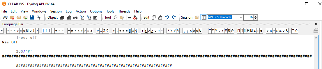
Fig. 7.2 Long output wrapping to the next line(s).#
Despite using the session width to automatically decide if the output is too wide or not, the user can have some control over that, even before bringing in ]rows to the table.
Through the system variable print width ⎕PW, the user can control the number of characters that are allowed per line before the output is wrapped onto the next line.
You can assign an integer in the range 42 to 32767 to the variable ⎕PW to change the print width of your session.
(We will take a more detailed look at system variables and functions later on.)
Let us create a dfn that produces a simple ruler to measure our session:
ruler ← {⍵⍴'----''----|'}
And let us use it to explore what happens with output that is “too long”, as per what the print width determines is too long:
⎕PW ← 50
ruler 50
ruler 51
We can see that lines that are longer than ⎕PW characters get wrapped and indented.
When you produce (really) long outputs, it can be unwieldy to have the output wrap to new lines, so one might think about increasing the value of the print width variable:
⎕PW ← 60
ruler 51
Now we don’t have to scroll vertically to get past the output of this single expression.
With ]rows we can get a similar effect, with the added benefit that we do not have to set the print width manually.
Notice that ]rows takes care of ensuring that the output does not wrap to the next line(s):
]rows on
ruler 80
In fact, with ]rows on, the print width variable is no longer relevant, and the user command calculates the current screen width when needed.
But the user command ]rows can do much more than this; just remember that the help message showed a series of command modifiers that we haven’t explored yet.
Let us ask for a more detailed help description with -??:
]rows -??
Take your time to try to understand what the modifiers do, both by reading the help description above and by playing around with the modifiers in your session.
After you explore things on your own for a bit, indulge me in a brief overview of the several modifiers that ]rows accepts.
We start by exploring the -style= modifier.
The default is to have -style=long, which makes the session output go beyond the screen width.
Again, when ]rows is on, this screen width is computed dynamically and does not depend on the print width ⎕PW variable.
If, instead, we use the -style=cut option, then the output is cut when it reaches the screen width, and it isn’t displayed at all, making it so that we never need to scroll horizontally.
Long output that is truncated in this way is marked (by default) with three dots “∙”.
Fig. 7.3 shows what the session looks like after running an expression that produces a line of output that is wider than the screen width.
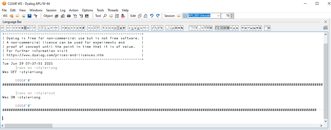
Fig. 7.3 A long line of session output with two different -style configurations.#
We can see that after setting -style=cut, the output was replaced with “∙∙∙” near the right edge of the screen.
If we scroll horizontally to the right, we can see that -style=long does allow the output to run beyond the screen and -style=cut effectively truncates it.
This is shown in Fig. 7.4, which is a screenshot from the exact same session output as above, except we have scrolled slightly to the right.
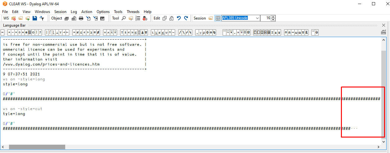
Fig. 7.4 A long line of output and the corresponding truncated version.#
Finally, the -style= modifier accepts one other option, which is -style=wrap.
This sets the behaviour of long lines to wrap to new lines, but this isn’t exactly the same as having ]rows off, because ]rows doesn’t rely on ⎕PW to figure out the screen width.
Notice how in the example below we have ⎕PW set to a small value that is disregarded by ]rows:
]rows on -style=wrap
⎕PW ← 50
ruler 60
Another difference between having ]rows off and ]rows on -style=wrap is that ]rows off will wrap the lines of output as a block, whereas -style=wrap will wrap each line individually, like Fig. 7.5 shows.
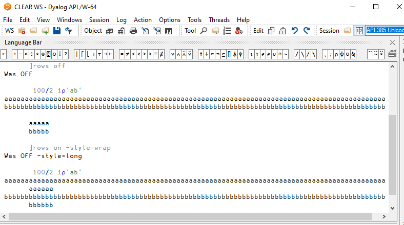
Fig. 7.5 Block wrapping versus individual line wrapping.#
Having looked at the different options for -style=, we are now left with three modifiers.
Just like the user command ]box, the user command ]rows only affects direct session output by default, and doesn’t affect function output.
This can be changed by setting the -fns= modifier:
]rows on -style=cut -fns=off
{v ← 500/'#' ⋄ ⎕← v ⋄ ⎕← '---' ⋄ v}⍬
As you can see above, the first output – that was produced by the ⎕← v statement inside the dfn – wrapped around because it was too long, effectively disregarding the modifier -style=cut from the user command ]rows.
However, the second run of # was truncated because it was the result of the expression that was typed in the session and it was too long.
We have been worrying about the horizontal space that output takes up, but some output can take up too much vertical space.
The user command ]rows can also be used to deal with that, and that is what the modifier -fold= is for.
If you set the modifier -fold=n (to an integer between 0 and 9, inclusive), then vertically long output gets its middle rows truncated, leaving only the beginning and the final n rows.
The examples that follow show the differences in output when -fold= is set to different values:
]rows on -fold=0
⍳100 1
]rows -fold=3
⍳100 1
]rows -fold=9
⍳100 1
The final modifier that we have to discuss is -dots=, that allows to customise the character that is used to represent that output is truncated.
By default, the character used is “∙”, like we can see above.
Changing the value is simple:
]rows -dots=#
⍳100 1
It is advisable that you leave the modifier -dots= unchanged, or set it to a character that has the same properties that “∙” has: it is a character that doesn’t add much visual noise and it isn’t an ASCII character, meaning it is unlikely that the truncation marks from ]rows will be mistaken by actual output or vice-versa.
That is why we reset -dots= to its original value here:
]rows -dots=∙
Fig. 7.6 Dyalog APL programming is pure Art.#
7.5. The Specialist’s Section#
You will find here rare or complex usages of the concepts presented in this chapter, or discover extended explanations which need the knowledge of some symbols that will be seen much further in the book.
If you are exploring APL for the first time, skip this section and go to the next chapter.
7.5.1. Advanced Usages of Execute#
7.5.1.1. Name Conflict#
Suppose that we would like to switch two letters inside a word. Let us write a function which accepts the index of the letters to switch as its left argument, and the name of an existing variable as its right argument.
It is important to note that the function works on the name of the variable, not on its value:
]dinput
Exchange ← {
    v ← ⌽⍺
    text ← ⍵,'[⍺]←',⍵,'[v]'
    ⍎text
}
Now we create a character vector containing a word, call our function to exchange two characters, and then check the value of the variable again:
word ← 'moral'
3 5 Exchange 'word'
word
In our example, ⍵ was equal to 'word', so the statement that assigns to text was equivalent to text ← 'word[⍺]←word[v]'.
All is well up to now. But now, let us try again on another variable:
v ← 'rats'
1 2 Exchange 'v'
v
The result now is wrong, it should have been 'arts'.
The reason is that the assignment to text is equivalent to text ← 'v[⍺]←v[v]', but v is the name of a local variable in the function.
When the last statement is executed, it exchanges items inside the local variable, not in the global one, which remains unchanged!
In fact, if we call Exchange with larger indices, we get an INDEX ERROR because the local variable v only has two elements:
1 4 Exchange 'v'
⍎INDEX ERROR
Exchange[3] v[⍺]←v[v]
                  ∧
In other words, be careful when execute is expected to work on global names, as there may be a risk of conflict with local names.
In order to reduce this risk, programmers sometimes use complex and weird names for the local names in such functions.
Another alternative is to try and write your functions to not rely on ⍎ for this kind of things, as that creates code that is much harder to debug; instead, write functions that take arguments and return their results explicitly.
See, for example, Section 5.10.2.
7.5.1.2. Conditional Execution#
For many years, execute has been used to conditionally execute certain expressions in a function, through the pattern ⍎(condition)/'statement'.
If the condition is satisfied, compress returns the character string unchanged, and the statement is then executed. On the other hand, if the condition is not satisfied, compress returns an empty character vector and execute does nothing.
Here is an example that gives a higher discount to customers that buy in bulk:
discount ← 0                     ⍝ default discount is 0
quantity ← 120
⍎(quantity>80)/'discount ← 7'
⎕← 'Final discount is ',⍕discount
This form is now considered obsolete and should be replaced by an :If ... :EndIf control structure.
There are also cases where it makes sense to rework the logic of the program slightly, so that the conditional and the resulting value are coupled together.
Going back to the previous example, one can use basic arithmetic operations to assign the correct discount value from the get-go:
quantity ← 120
discount ← (quantity>80)×7
⎕← 'Final discount is ',⍕discount
7.5.1.3. Case Selection#
Execute is sometimes used to select one case from a set of cases.
Consider the following scenario: a program allows the user to extrapolate a series of numeric values.
He has the choice between three extrapolation methods: least squares, moving average, and a home-made method.
Each can be applied using one of three functions: LeastSqr, MovAverage, HomeXtra.
We want to write a function that takes the method number (1 to 3) as its left argument, and the values to extrapolate as the right argument.
You can compare two programming techniques:
∇ r ← method Calc1 values
    :Select method
    :Case 1
        r ← LeastSqr values
    :Case 2
        r ← MovAverage values
    :Case 3
        r ← HomeXtra values
    :EndSelect
∇
∇ r ← method Calc2 values; fun
    fun ← (3 11⍴'LeastSqr   MovAverage HomeXtra   ')[method;]
    r ← ⍕fun,' values'
∇
Let us analyse how Calc2 works: suppose that the user has chosen the third method.
The assignment to fun evaluates to the character vector 'HomeXtra '.
Once this character vector is catenated to ' values' we obtain 'HomeXtra values'.
Then, execute calls the appropriate function and returns the desired result.
This form too is considered obsolete and should be avoided, if only for clarity.
7.5.1.4. Dynamic Variable Creation#
Some very specific applications may require that a program creates variables whose names depend on the context. This may seem a bit artificial, but imagine that we have three variables:
prefixis the following text matrix:
⎕← prefix ← 4 8⍴'prod price discountorders '
suffixis a text vector:
⎕← suffix ← 'USA'
numbersis a numeric matrix:
numbers ← 4 4⍴623 486 739 648 108 103 112 98 7 6 7 5 890 942 637 806
Now we want to create variables named prodUSA, priceUSA, and so on, and fill them with the corresponding values.
A simple loop should do that:
∇ BuildVars (mat vec val); row; name
    :For row :In ⍳1↑⍴mat
        name ← mat[row;],vec
        name ← (name≠' ')/name
        ⍎ ⎕← name,'←val[row;]'
    :End
∇
Let us use the debugging output that we have added to the final line of the :For loop to see the code that is being executed by ⍎ on each iteration:
BuildVars (prefix suffix numbers)
This technique is prone to introduce errors that are hard to debug due to the dynamic nature of the variables being created.
Instead, one might consider leaving the values as-is, and using something like index of to determine dynamically the row of numbers that needs to be accessed.
For example, we could store the names of the rows as a nested character vector:
⎕← rowNames ← 'prod' 'price' 'discount' 'orders'
And then use that variable to determine what is the row of numbers we need to access:
numbers[rowNames⍳⊂'prod';]
This approach is also easy to extend if, instead of a single country in the variable suffix, we had a series of countries:
countries ← 'USA' 'Canada' 'Portugal'
Which could be accompanied by a larger numbers matrix; in fact, we could even have a 3D array where each sub-matrix corresponds to one country:
⎕← numbers ← 3 4 4⍴623 486 739 648 108 103 112 98 7 6 7 5 890 942 637 806 646 502 778 670 114 105 122 102 8 7 8 6 903 980 688 844 675 531 767 667 114 110 117 108 8 7 8 6 906 993 689 824
Then, we could use a similar technique to access the production of a single country, instead of dynamically creating 12 different variables:
numbers[countries⍳⊂'Portugal';rowNames⍳⊂'prod';]
7.5.1.5. Dyadic Execute#
In the dyadic use of execute, the left argument can be the name of a namespace or a namespace reference. The statement provided as the right argument will then be executed in the namespace specified as the left argument.
For example, we can do a dynamic assignment to the global scope from within a dfn:
'var' {'#'⍎⍺,' ← ',⍕⍵} 42
var
Instead of '#' we can use the actual namespace reference:
'var' {#⍎⍺,' ← ',⍕⍵} 73
var
With the left argument being a namespace reference, you can also do “zero footprint” execution with (⎕NS⍬)⍎expr, where expr is what you want to execute.
Here, “zero footprint” means that after the expression is executed, nothing remains, other than the things that the expression explicitly did/built outside of its namespace.
7.5.2. Formatting Data#
7.5.2.1. Lack of Precision#
If the number of specified significant digits exceeds the computer’s internal precision, low order digits are replaced with an underscore (_).
This character can be replaced by another one using specification 'S'.
For example:
'F20.1' ⎕FMT 1e18÷3
'S⊂_?⊃F20.1' ⎕FMT 1e18÷3
7.5.2.2. Formatting Using the Microsoft .NET Framework#
Dyalog APL has an interface to Microsoft’s .NET framework, which is introduced in a later chapter. The .NET framework includes a vast collection of utility programs, including functions to interpret and format data according to rules defined for a given locale, or culture, or language (which you can customise on your operating system).
Let us start by declaring our intent to use the .NET framework:
⎕USING ← ''
Then let us do a quick check to see if it loaded:
System.Math.BigMul 1e9 1e9
Now we illustrate some of the capabilities of the String.Format method.
The String.Format function takes three arguments: an instance of the NumberFormatInfo class, a format string, and a vector of data.
An appropriate NumberFormatInfo instance can be retrieved from an object that contains information about the current culture of the system.
We start by querying for the current culture:
⎕← cc ← System.Globalization.CultureInfo.CurrentCulture
cc.EnglishName
Now we can call the String.Format method, that returns a string, which appears in APL as a character vector:
pi ← ○1
System.String.Format cc.NumberFormat '{0:F}' (,pi)
The 0 in {0:F} is an index (selecting the first item in the data array), and F specifies fixed-point formatting.
The default number of digits and the decimal separator to use are specified in the NumberFormatInfo object, which has a number of properties that we can inspect, if we need to know more about how numbers are formatted in the selected culture:
cc.NumberFormat.(NumberDecimalSeparator NumberDecimalDigits)
Of course, we don’t have to use the default format; we can also specify the number of decimal digits that we want.
In the following string we format the first number as a fixed-point number with 5 decimal digits and the second as a currency amount with 2 digits (C2):
format ← 'Pi is {0:F5} and I have {1:C2}'
System.String.Format cc.NumberFormat format (pi×1 2)
We also don’t have to use the current culture, we can select any of the cultures known to the .NET framework:
fr ← ⎕NEW System.Globalization.CultureInfo (⊂'fr-FR')
System.String.Format fr.NumberFormat format (pi×1 2)
We can format dates:
⎕← jun29 ← ⎕NEW System.DateTime (2021 6 29 17 40 0)
System.String.Format cc.NumberFormat '{0:D}' (,jun29)
There is also a wide variety of options and parameters for formatting dates, for example:
format ← 'Short date: {0:d}, custom date: {0:dd MMMM yy hh:mm}'
System.String.Format cc.NumberFormat format (,jun29)
In the case of dates (and many other classes), the System.DateTime class itself has a toString method which hooks up to the same underlying functionality:
jun29.ToString '{yyyy, dd MMMM}' fr
jun29.ToString ⊂'{dd MMMM yy}'
The .NET base classes generally also contain a function called Parse, which performs the inverse operation:
System.Double.Parse ⊂'3.14'
System.Double.Parse '3,14' fr
System.DateTime.Parse ⊂'29 june 2021 17:40'
The examples above have only scratched the surface of the wide variety of formatting options which are available. More documentation of the available formatting options is available online at https://docs.microsoft.com (search for “formatting types”).
The related system function ⎕DT might also be relevant if you are particularly interested in working with dates/times.